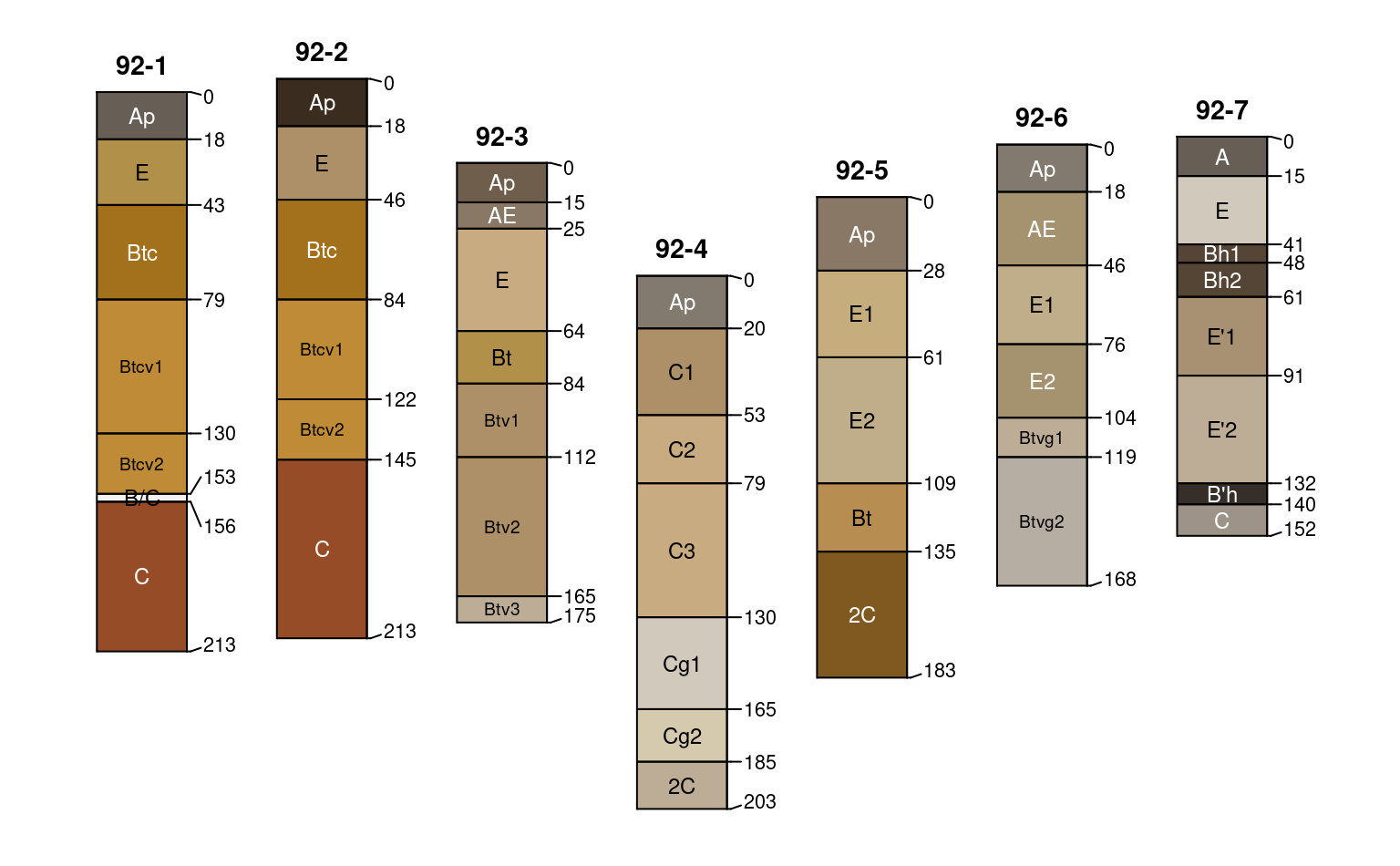
Generate a diagram of soil profile sketches from a SoilProfileCollection object. The Introduction to SoilProfileCollection Objects Vignette contains many examples and discussion of the large number of arguments to this function. The Soil Profile Sketches tutorial has longer-form discussion and examples pertaining to suites of related arguments.
Options can be used to conveniently specify sets of arguments that will be used in several calls to plotSPC() within a single R session. For example, arguments can be specified in a named list (.a) and set using: options(.aqp.plotSPC.args = .a). Reset these options via options(.aqp.plotSPC.args = NULL). Arguments explicitly passed to plotSPC() will override arguments set via options().
Usage
plotSPC(
  x,
  color = "soil_color",
  width = ifelse(length(x) < 2, 0.15, 0.25),
  name = hzdesgnname(x),
  name.style = "right-center",
  label = idname(x),
  raggedBottom = NULL,
  hz.depths = FALSE,
  hz.depths.offset = ifelse(fixLabelCollisions, 0.03, 0),
  hz.depths.lines = fixLabelCollisions,
  depth.axis = list(style = "traditional", cex = cex.names * 1.15),
  alt.label = NULL,
  alt.label.col = "black",
  cex.names = 0.5,
  cex.id = cex.names + (0.2 * cex.names),
  font.id = 2,
  srt.id = 0,
  offset.id = 0.5,
  print.id = TRUE,
  id.style = "auto",
  plot.order = 1:length(x),
  relative.pos = 1:length(x),
  add = FALSE,
  scaling.factor = 1,
  y.offset = rep(0, times = length(x)),
  x.idx.offset = 0,
  n = length(x),
  max.depth = ifelse(is.infinite(max(x)), 200, max(x)),
  n.depth.ticks = 10,
  shrink = FALSE,
  shrink.cutoff = 3,
  shrink.thin = NULL,
  abbr = FALSE,
  abbr.cutoff = 5,
  divide.hz = TRUE,
  hz.distinctness.offset = NULL,
  hz.topography.offset = NULL,
  hz.boundary.lty = NULL,
  density = NULL,
  show.legend = TRUE,
  col.label = color,
  col.palette = c("#5E4FA2", "#3288BD", "#66C2A5", "#ABDDA4", "#E6F598", "#FEE08B",
    "#FDAE61", "#F46D43", "#D53E4F", "#9E0142"),
  col.palette.bias = 1,
  col.legend.cex = 1,
  n.legend = 8,
  lwd = 1,
  lty = 1,
  default.color = grey(0.95),
  fixLabelCollisions = hz.depths,
  fixOverlapArgs = list(method = "E", q = 1),
  cex.depth.axis = cex.names,
  axis.line.offset = -2,
  plot.depth.axis = TRUE,
  ...
)

# S4 method for class 'SoilProfileCollection'
plot(x, y, ...)
Arguments
- x
a
SoilProfileCollectionobject- color
quoted column name containing R-compatible color descriptions, or numeric / categorical data to be displayed thematically; see details
- width
scaling of profile widths (typically 0.1 - 0.4)
- name
quoted column name of the (horizon-level) attribute containing horizon designations or labels, if missing
hzdesgnname(x)is used. Suppress horizon name printing by settingname = NAorname = ''.- name.style
one of several possible horizon designations labeling styles:
c('right-center', 'left-center', 'left-top', 'center-center', 'center-top')- label
quoted column name of the (site-level) attribute used to identify profile sketches
- raggedBottom
either quoted column name of the (site-level) attribute (logical) used to mark profiles with a truncated lower boundary, or
FALSEsuppress ragged bottom depths whenmax.depth < max(x)- hz.depths
logical, annotate horizon top depths to the right of each sketch (
FALSE)- hz.depths.offset
numeric, user coordinates for left-right adjustment for horizon depth annotation; reasonable values are usually within 0.01-0.05 (default: 0)
- hz.depths.lines
logical, draw segments between horizon depth labels and actual horizon depth; this is useful when including horizon boundary distinctness and/or
fixLabelCollisions = TRUE- depth.axis
logical or list. Use a logical to suppress (
FALSE) or add depth axis using defaults (TRUE). Use a list to specify one or more of:style: character, one of 'traditional', 'compact', or 'tape'line: numeric, negative values move axis to the left (does not apply tostyle = 'tape')cex: numeric, scaling applied to entire depth axisinterval: numeric, axis interval See examples.
- alt.label
quoted column name of the (site-level) attribute used for secondary annotation
- alt.label.col
color used for secondary annotation text
- cex.names
baseline character scaling applied to all text labels
- cex.id
character scaling applied to
label- font.id
font style applied to
label, default is 2 (bold)- srt.id
rotation applied to
label, only whenid.style = 'top'- offset.id
vertical offset applied to
label, only whenid.style = 'top'- print.id
logical, print
labelabove/beside each profile? (TRUE)- id.style
labelprinting style: 'auto' (default) = simple heuristic used to select from: 'top' = centered above each profile, 'side' = 'along the top-left edge of profiles'- plot.order
integer vector describing the order in which individual soil profiles should be plotted
- relative.pos
vector of relative positions along the x-axis, within {1, n}, ignores
plot.ordersee details- add
logical, add to an existing figure
- scaling.factor
vertical scaling of profile depths, useful for adding profiles to an existing figure
- y.offset
numeric vector of vertical offset for top of profiles in depth units of
x, can either be a single numeric value or vector of length =length(x). A vector of y-offsets will be automatically re-ordered according toplot.order.- x.idx.offset
integer specifying horizontal offset from 0 (left-hand edge)
- n
integer describing amount of space along x-axis to allocate, defaults to
length(x)- max.depth
numeric. The lower depth for all sketches, deeper profiles are truncated at this depth. Use larger values to arbitrarily extend the vertical dimension, convenient for leaving extract space for annotation.
- n.depth.ticks
suggested number of ticks in depth scale
- shrink
logical, reduce character scaling for 'long' horizon by 80%
- shrink.cutoff
character length defining 'long' horizon names
- shrink.thin
integer, horizon thickness threshold for shrinking horizon names by 80%, only activated when
shrink = TRUE(NULL= no shrinkage)- abbr
logical, abbreviate
label- abbr.cutoff
suggested minimum length for abbreviated
label- divide.hz
logical, divide horizons with line segment? (
TRUE), see details- hz.distinctness.offset
NULL, or quoted column name (horizon-level attribute) containing vertical offsets used to depict horizon boundary distinctness (same units as profiles), see details andhzDistinctnessCodeToOffset(); consider settinghz.depths.lines = TRUEwhen used in conjunction withhz.depths = TRUE- hz.topography.offset
NULL, or quoted column name (horizon-level attribute) containing offsets used to depict horizon boundary topography (same units as profiles), see details andhzTopographyCodeToOffset()- hz.boundary.lty
quoted column name (horizon-level attribute) containing line style (integers) used to encode horizon topography
- density
fill density used for horizon color shading, either a single integer or a quoted column name (horizon-level attribute) containing integer values (default is
NULL, no shading)- show.legend
logical, show legend? (default is
TRUE)- col.label
thematic legend title
- col.palette
color palette used for thematic sketches (default is
rev(brewer.pal(10, 'Spectral')))- col.palette.bias
color ramp bias (skew), see
colorRamp()- col.legend.cex
scaling of thematic legend
- n.legend
approximate number of classes used in numeric legend, max number of items per row in categorical legend
- lwd
line width multiplier used for sketches
- lty
line style used for sketches
- default.color
default horizon fill color used when
colorattribute isNA- fixLabelCollisions
use
fixOverlap()to attempt fixing hz depth labeling collisions, will slow plotting of large collections; enabling also setshz.depths.lines = TRUE. Additional arguments tofixOverlap()can be passed viafixOverlapArgs. Overlap collisions cannot be fixed within profiles containing degenerate or missing horizon depths (e.g. top == bottom).- fixOverlapArgs
a named list of arguments to
fixOverlap(). Overlap adjustments are attempted using electrostatic simulation with arguments:list(method = 'E', q = 1). Alternatively, select adjustment by simulated annealing vialist(method = 'S'). SeeelectroStatics_1D()andSANN_1D()for details.- cex.depth.axis
(deprecated, use
depth.axisinstead) character scaling applied to depth scale- axis.line.offset
(deprecated, use
depth.axisinstead) horizontal offset applied to depth axis (default is -2, larger numbers move the axis to the right)- plot.depth.axis
(deprecated, use
depth.axisinstead) logical, plot depth axis?- ...
other arguments passed into lower level plotting functions
- y
(not used)
Details
Depth limits (max.depth) and number of depth ticks (n.depth.ticks) are suggestions to the pretty() function. You may have to tinker with both parameters to get what you want.
The 'side' id.style is useful when plotting a large collection of profiles, and/or, when profile IDs are long.
If the column containing horizon designations is not specified (the name argument), a column (presumed to contain horizon designation labels) is guessed based on regular expression matching of the pattern 'name'–this usually works, but it is best to manual specify the name of the column containing horizon designations.
The color argument can either name a column containing R-compatible colors, possibly created via munsell2rgb(), or column containing either numeric or categorical (either factor or character) values. In the second case, values are converted into colors and displayed along with a simple legend above the plot. Note that this functionality makes several assumptions about plot geometry and is most useful in an interactive setting.
Adjustments to the legend can be specified via col.label (legend title), col.palette (palette of colors, automatically expanded), col.legend.cex (legend scaling), and n.legend (approximate number of classes for numeric variables, or, maximum number of legend items per row for categorical variables). Currently, plotSPC will only generate two rows of legend items. Consider reducing the number of classes if two rows isn't enough room.
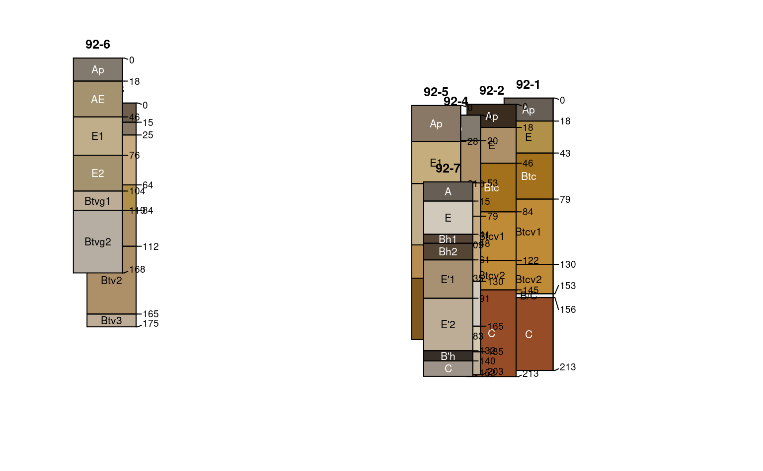
Profile sketches can be added according to relative positions along the x-axis (vs. integer sequence) via relative.pos argument. This should be a vector of positions within {1,n} that are used for horizontal placement. Default values are 1:length(x). Care must be taken when both plot.order and relative.pos are used simultaneously: relative.pos specifies horizontal placement after sorting. addDiagnosticBracket() and addVolumeFraction() use the relative.pos values for subsequent annotation.
Relative positions that are too close will result in overplotting of sketches. Adjustments to relative positions such that overlap is minimized can be performed with fixOverlap(pos), where pos is the original vector of relative positions.
The x.idx.offset argument can be used to shift a collection of pedons from left to right in the figure. This can be useful when plotting several different SoilProfileCollection objects within the same figure. Space must be pre-allocated in the first plotting call, with an offset specified in the second call. See examples below.
Horizon depths (e.g. cm) are converted to figure y-coordinates via: y = (depth * scaling.factor) + y.offset.
References
Beaudette, D.E., Roudier P., and A.T. O'Geen. 2013. Algorithms for Quantitative Pedology: A Toolkit for Soil Scientists. Computers & Geosciences. 52:258 - 268.
Examples
# keep examples from using more than 2 cores
data.table::setDTthreads(Sys.getenv("OMP_THREAD_LIMIT", unset = 2))
# example data
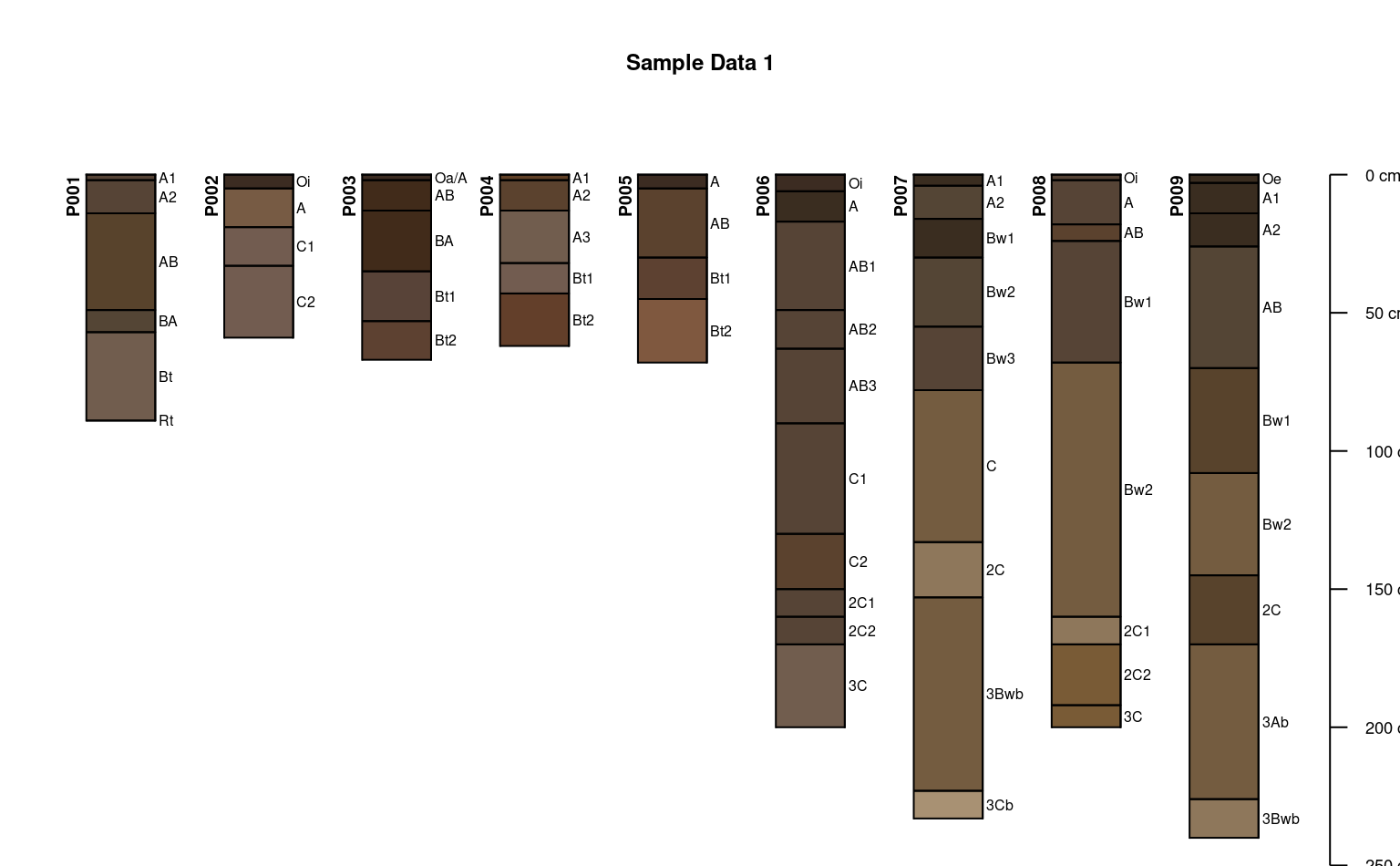
data(sp1)
# usually best to adjust margins
par(mar = c(0,0,3,0))
# add color vector
sp1$soil_color <- with(sp1, munsell2rgb(hue, value, chroma))
# promote to SoilProfileCollection
depths(sp1) <- id ~ top + bottom
# init horizon designation
hzdesgnname(sp1) <- 'name'
# plot profiles
plotSPC(sp1, id.style = 'side')
# title, note line argument:
title('Sample Data 1', line = 1, cex.main = 0.75)
 # plot profiles without horizon-line divisions
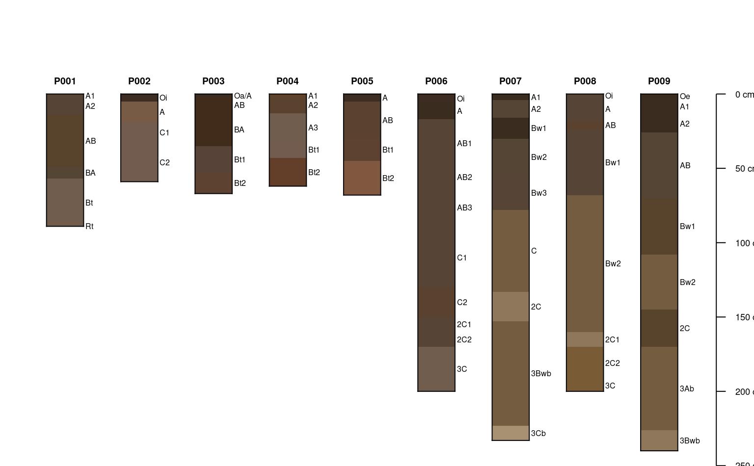
plotSPC(sp1, divide.hz = FALSE)
# plot profiles without horizon-line divisions
plotSPC(sp1, divide.hz = FALSE)
 # diagonal lines encode horizon boundary distinctness
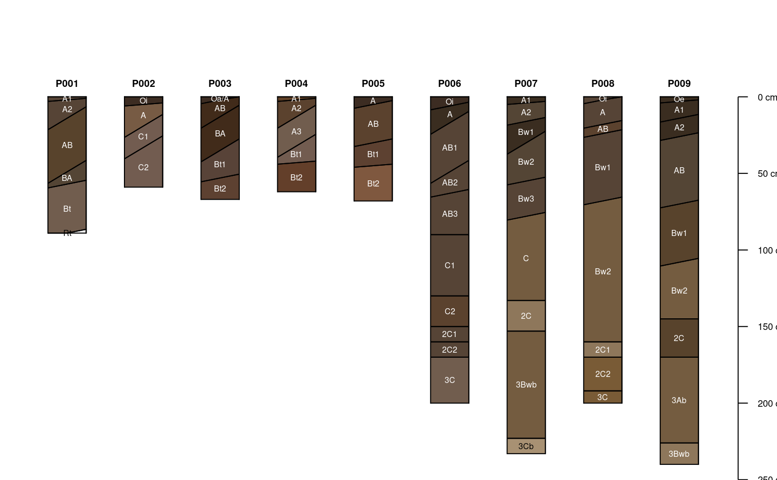
sp1$hzD <- hzDistinctnessCodeToOffset(sp1$bound_distinct)
plotSPC(sp1, hz.distinctness.offset = 'hzD', name.style = 'center-center')
# diagonal lines encode horizon boundary distinctness
sp1$hzD <- hzDistinctnessCodeToOffset(sp1$bound_distinct)
plotSPC(sp1, hz.distinctness.offset = 'hzD', name.style = 'center-center')
 # plot horizon color according to some property
data(sp4)
depths(sp4) <- id ~ top + bottom
hzdesgnname(sp4) <- 'name'
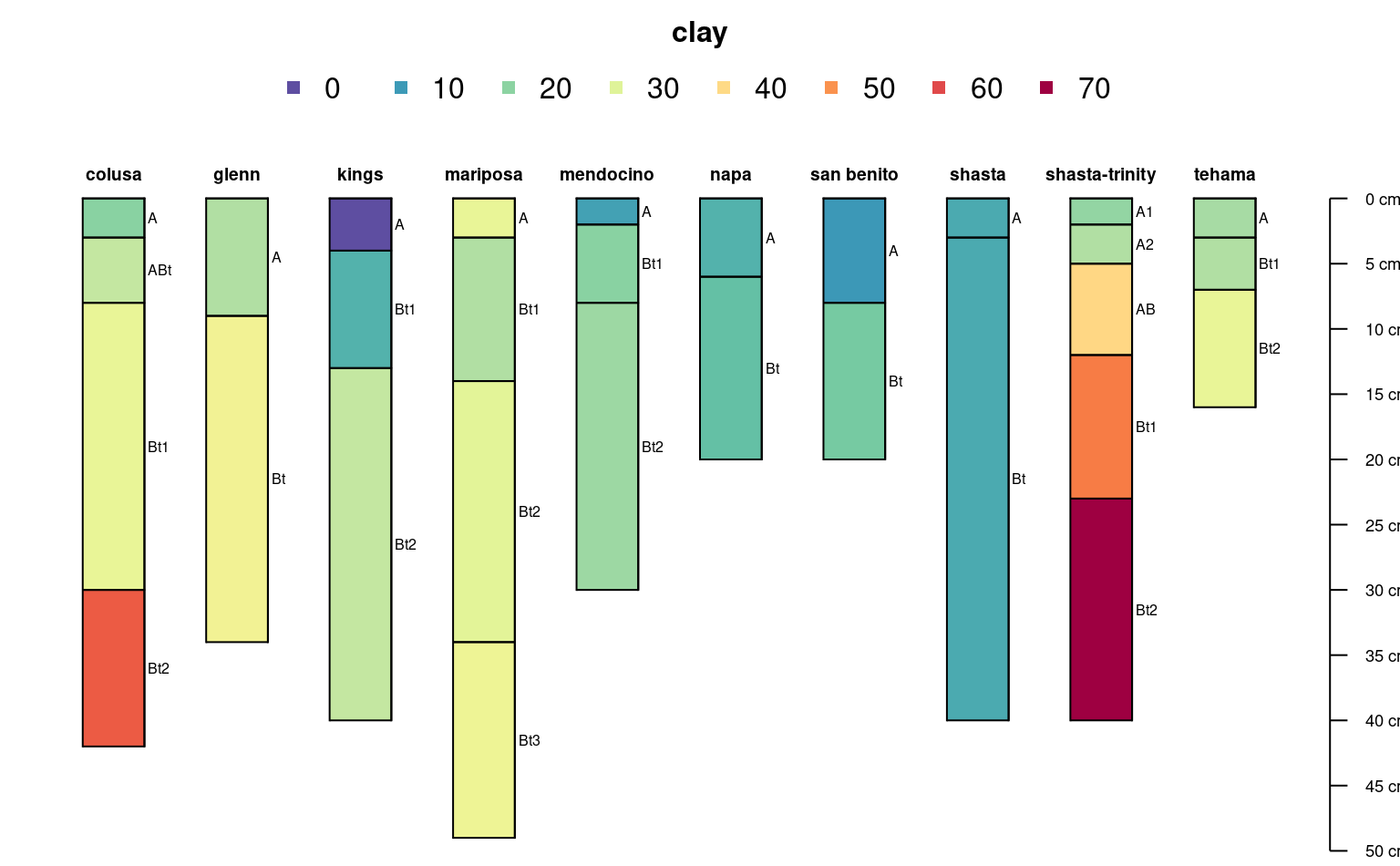
plotSPC(sp4, color = 'clay')
# plot horizon color according to some property
data(sp4)
depths(sp4) <- id ~ top + bottom
hzdesgnname(sp4) <- 'name'
plotSPC(sp4, color = 'clay')
 # another example
data(sp2)
depths(sp2) <- id ~ top + bottom
hzdesgnname(sp2) <- 'name'
site(sp2) <- ~ surface
# some of these profiles are very deep, truncate plot at 400cm
# label / re-order with site-level attribute: `surface`
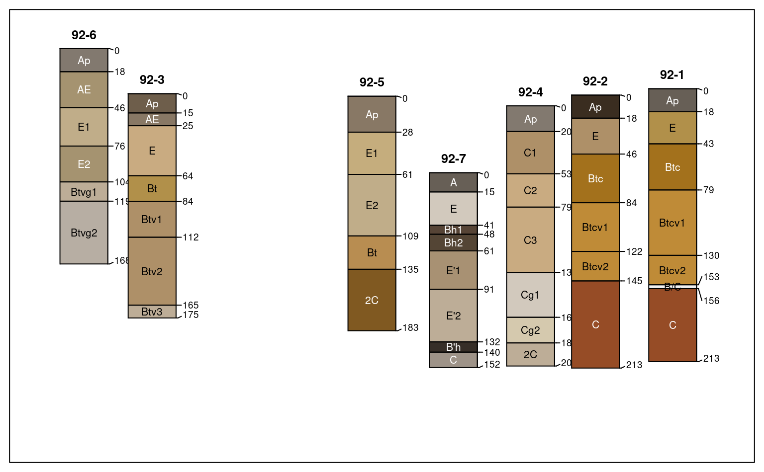
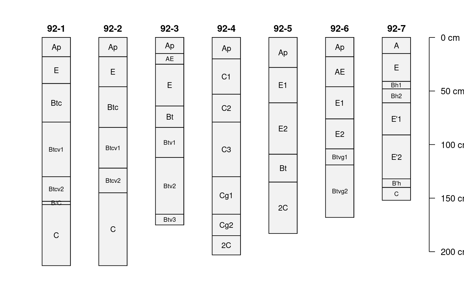
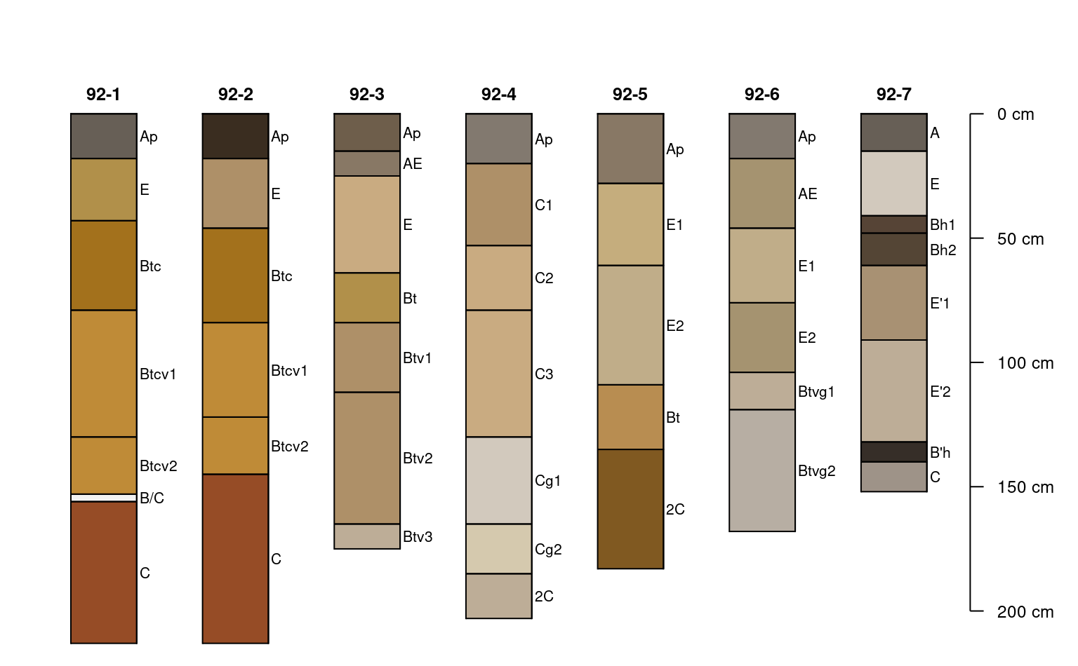
plotSPC(sp2, label = 'surface', plot.order = order(sp2$surface),
max.depth = 400)
# another example
data(sp2)
depths(sp2) <- id ~ top + bottom
hzdesgnname(sp2) <- 'name'
site(sp2) <- ~ surface
# some of these profiles are very deep, truncate plot at 400cm
# label / re-order with site-level attribute: `surface`
plotSPC(sp2, label = 'surface', plot.order = order(sp2$surface),
max.depth = 400)
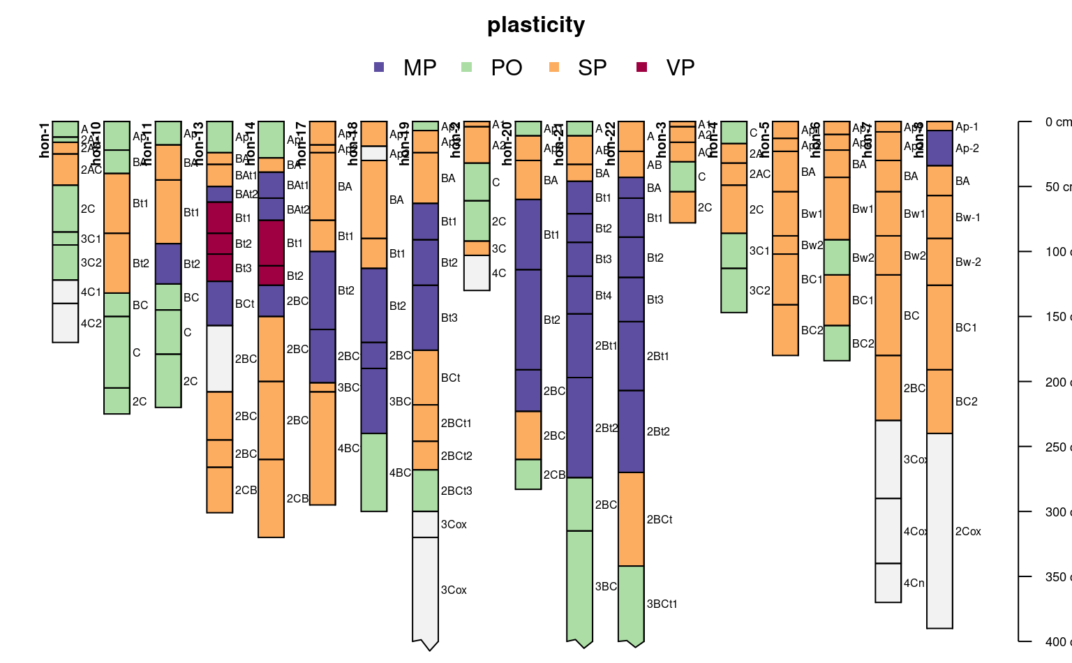
 # example using a categorical attribute
plotSPC(sp2, color = "plasticity",
max.depth = 400)
# example using a categorical attribute
plotSPC(sp2, color = "plasticity",
max.depth = 400)
 # plot two SPC objects in the same figure
par(mar = c(1,1,1,1))
# plot the first SPC object and
# allocate space for the second SPC object
plotSPC(sp1, n = length(sp1) + length(sp2))
# plot the second SPC, starting from the first empty space
plotSPC(sp2, x.idx.offset = length(sp1), add = TRUE)
# plot two SPC objects in the same figure
par(mar = c(1,1,1,1))
# plot the first SPC object and
# allocate space for the second SPC object
plotSPC(sp1, n = length(sp1) + length(sp2))
# plot the second SPC, starting from the first empty space
plotSPC(sp2, x.idx.offset = length(sp1), add = TRUE)
 ##
## demonstrate horizon designation shrinkage
##
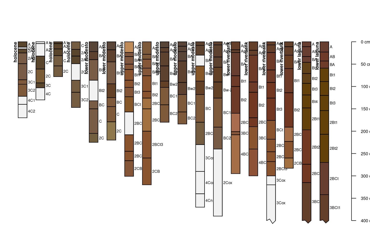
data("jacobs2000")
# shrink "long" horizon names
plotSPC(
jacobs2000,
name = 'name',
name.style = 'center-center',
shrink = TRUE,
cex.names = 0.8
)
##
## demonstrate horizon designation shrinkage
##
data("jacobs2000")
# shrink "long" horizon names
plotSPC(
jacobs2000,
name = 'name',
name.style = 'center-center',
shrink = TRUE,
cex.names = 0.8
)
 # shrink horizon names in "thin" horizons
plotSPC(
jacobs2000,
name = 'name',
name.style = 'center-center',
shrink = TRUE,
shrink.thin = 15,
cex.names = 0.8,
)
# shrink horizon names in "thin" horizons
plotSPC(
jacobs2000,
name = 'name',
name.style = 'center-center',
shrink = TRUE,
shrink.thin = 15,
cex.names = 0.8,
)
 ##
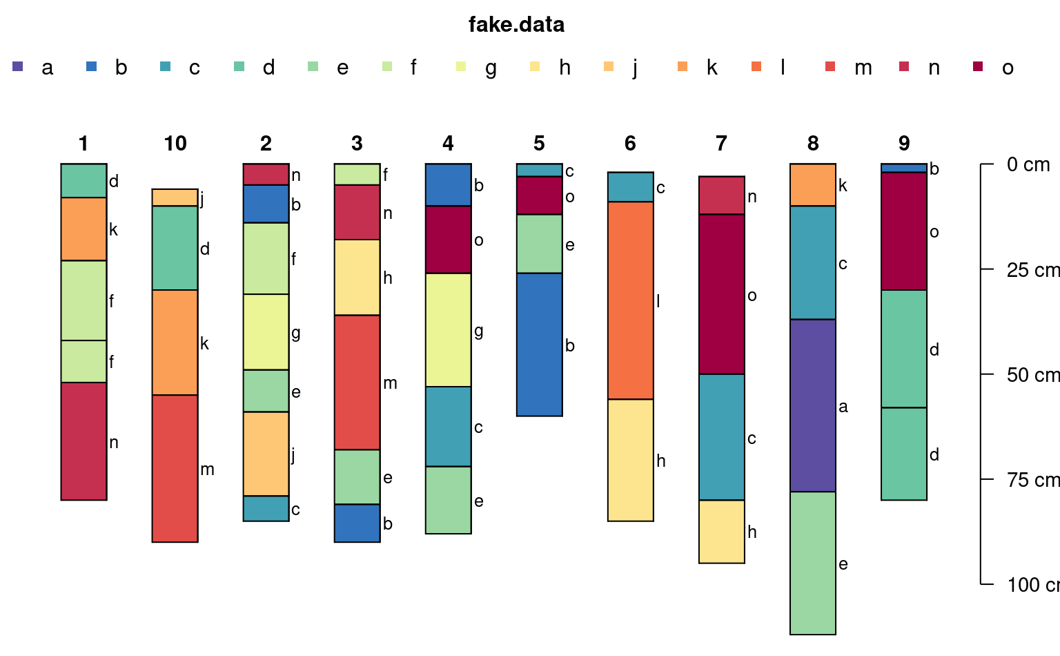
## demonstrate adaptive legend
##
data(sp3)
depths(sp3) <- id ~ top + bottom
# make some fake categorical data
horizons(sp3)$fake.data <- sample(letters[1:15], size = nrow(sp3), replace=TRUE)
# better margins
par(mar=c(0,0,3,1))
# note that there are enough colors for 15 classes (vs. previous limit of 10)
# note that the legend is split into 2 rows when length(classes) > n.legend argument
plotSPC(sp3, color='fake.data', name='fake.data', cex.names=0.8)
##
## demonstrate adaptive legend
##
data(sp3)
depths(sp3) <- id ~ top + bottom
# make some fake categorical data
horizons(sp3)$fake.data <- sample(letters[1:15], size = nrow(sp3), replace=TRUE)
# better margins
par(mar=c(0,0,3,1))
# note that there are enough colors for 15 classes (vs. previous limit of 10)
# note that the legend is split into 2 rows when length(classes) > n.legend argument
plotSPC(sp3, color='fake.data', name='fake.data', cex.names=0.8)
 # make enough room in a single legend row
plotSPC(sp3, color='fake.data', name='fake.data', cex.names=0.8, n.legend=15)
# make enough room in a single legend row
plotSPC(sp3, color='fake.data', name='fake.data', cex.names=0.8, n.legend=15)
 ##
## demonstrate y.offset argument
## must be of length 1 or length(x)
##
# example data and local copy
data("jacobs2000")
x <- jacobs2000
hzdesgnname(x) <- 'name'
# y-axis offsets, simulating a elevation along a hillslope sequence
# same units as horizon depths in `x`
# same order as profiles in `x`
y.offset <- c(-5, -10, 22, 65, 35, 15, 12)
par(mar = c(0, 0, 2, 2))
# y-offset at 0
plotSPC(x, color = 'matrix_color', cex.names = 0.66)
##
## demonstrate y.offset argument
## must be of length 1 or length(x)
##
# example data and local copy
data("jacobs2000")
x <- jacobs2000
hzdesgnname(x) <- 'name'
# y-axis offsets, simulating a elevation along a hillslope sequence
# same units as horizon depths in `x`
# same order as profiles in `x`
y.offset <- c(-5, -10, 22, 65, 35, 15, 12)
par(mar = c(0, 0, 2, 2))
# y-offset at 0
plotSPC(x, color = 'matrix_color', cex.names = 0.66)
 # constant adjustment to y-offset
plotSPC(x, color = 'matrix_color', cex.names = 0.66, y.offset = 50)
# constant adjustment to y-offset
plotSPC(x, color = 'matrix_color', cex.names = 0.66, y.offset = 50)
 # attempt using invalid y.offset
# warning issued and default value of '0' used
# plotSPC(x, color = 'matrix_color', cex.names = 0.66, y.offset = 1:2)
# variable y-offset
# fix overlapping horizon depth labels
par(mar = c(0, 0, 1, 0))
plotSPC(
x,
y.offset = y.offset,
color = 'matrix_color',
cex.names = 0.75,
shrink = TRUE,
hz.depths = TRUE,
hz.depths.offset = 0.05,
fixLabelCollisions = TRUE,
name.style = 'center-center'
)
# attempt using invalid y.offset
# warning issued and default value of '0' used
# plotSPC(x, color = 'matrix_color', cex.names = 0.66, y.offset = 1:2)
# variable y-offset
# fix overlapping horizon depth labels
par(mar = c(0, 0, 1, 0))
plotSPC(
x,
y.offset = y.offset,
color = 'matrix_color',
cex.names = 0.75,
shrink = TRUE,
hz.depths = TRUE,
hz.depths.offset = 0.05,
fixLabelCollisions = TRUE,
name.style = 'center-center'
)
 #> depth axis is disabled when more than 1 unique y offsets are supplied
# random y-axis offsets
yoff <- runif(n = length(x), min = 1, max = 100)
# random gradient of x-positions
xoff <- runif(n = length(x), min = 1, max = length(x))
# note profiles overlap
plotSPC(x,
relative.pos = xoff,
y.offset = yoff,
color = 'matrix_color',
cex.names = 0.66,
hz.depths = TRUE,
name.style = 'center-center'
)
#> depth axis is disabled when more than 1 unique y offsets are supplied
# random y-axis offsets
yoff <- runif(n = length(x), min = 1, max = 100)
# random gradient of x-positions
xoff <- runif(n = length(x), min = 1, max = length(x))
# note profiles overlap
plotSPC(x,
relative.pos = xoff,
y.offset = yoff,
color = 'matrix_color',
cex.names = 0.66,
hz.depths = TRUE,
name.style = 'center-center'
)
 #> depth axis is disabled when more than 1 unique y offsets are supplied
# align / adjust relative x positions
set.seed(111)
pos <- alignTransect(xoff, x.min = 1, x.max = length(x), thresh = 0.65)
#> 136 iterations
# y-offset is automatically re-ordered according to
# plot.order
par(mar = c(0.5, 0.5, 0.5, 0.5))
plotSPC(x,
plot.order = pos$order,
relative.pos = pos$relative.pos,
y.offset = yoff,
color = 'matrix_color',
cex.names = 0.66,
hz.depths = TRUE,
name.style = 'center-center'
)
#> depth axis is disabled when more than 1 unique y offsets are supplied
box()
#> depth axis is disabled when more than 1 unique y offsets are supplied
# align / adjust relative x positions
set.seed(111)
pos <- alignTransect(xoff, x.min = 1, x.max = length(x), thresh = 0.65)
#> 136 iterations
# y-offset is automatically re-ordered according to
# plot.order
par(mar = c(0.5, 0.5, 0.5, 0.5))
plotSPC(x,
plot.order = pos$order,
relative.pos = pos$relative.pos,
y.offset = yoff,
color = 'matrix_color',
cex.names = 0.66,
hz.depths = TRUE,
name.style = 'center-center'
)
#> depth axis is disabled when more than 1 unique y offsets are supplied
box()