Introduction to SoilProfileCollection Objects

Introduction

This is a basic introduction to the SoilProfileCollection class object defined in the aqp package for R.

The SoilProfileCollection class was designed to simplify the process of working with the collection of data associated with soil profiles: site-level data, horizon-level data, spatial data, diagnostic horizon data, metadata, etc.

Examples listed below are meant to be copied/pasted from this document and interactively run within R. Comments (preceded by # symbol) briefly describe what the code in each line does. Further documentation on objects and functions from the aqp package can be accessed by typing help(aqp) (or more generally, ?function_name) at the R console.

Setup

In this tutorial we will use some sample data included with the aqp package, based on characterization data from 10 soils sampled on serpentinitic parent material as described in McGahan et al, 2009.

To begin you will load required packages. You may have to first install these if missing:

# install CRAN release + dependencies
install.packages('aqp', dependencies = TRUE)
install.packages('remotes', dependencies = TRUE)

# install latest version from GitHub
remotes::install_github("ncss-tech/aqp", dependencies = FALSE)

library(aqp)
library(lattice)

# load sample data set, a data.frame object with horizon-level data from 10 profiles
data(sp4)
str(sp4)

#> 'data.frame':    30 obs. of  13 variables:
#>  $ id         : chr  "colusa" "colusa" "colusa" "colusa" ...
#>  $ name       : chr  "A" "ABt" "Bt1" "Bt2" ...
#>  $ top        : int  0 3 8 30 0 9 0 4 13 0 ...
#>  $ bottom     : int  3 8 30 42 9 34 4 13 40 6 ...
#>  $ K          : num  0.3 0.2 0.1 0.1 0.2 0.3 0.2 0.6 0.8 0.4 ...
#>  $ Mg         : num  25.7 23.7 23.2 44.3 21.9 18.9 12.1 12.1 17.7 16.4 ...
#>  $ Ca         : num  9 5.6 1.9 0.3 4.4 4.5 1.4 7 4.4 24.1 ...
#>  $ CEC_7      : num  23 21.4 23.7 43 18.8 27.5 23.7 18 20 31.1 ...
#>  $ ex_Ca_to_Mg: num  0.35 0.23 0.08 0.01 0.2 0.2 0.58 0.51 0.25 1.47 ...
#>  $ sand       : int  46 42 40 27 54 49 43 36 27 43 ...
#>  $ silt       : int  33 31 28 18 20 18 55 49 45 42 ...
#>  $ clay       : int  21 27 32 55 25 34 3 15 27 15 ...
#>  $ CF         : num  0.12 0.27 0.27 0.16 0.55 0.84 0.5 0.75 0.67 0.02 ...

# optionally read about it...
# ?sp4

# upgrade to SoilProfileCollection
# 'id' is the name of the column containing the profile ID
# 'top' is the name of the column containing horizon upper boundaries
# 'bottom' is the name of the column containing horizon lower boundaries
depths(sp4) <- id ~ top + bottom

# define "horizon designation" column name for the collection
hzdesgnname(sp4) <- 'name'

# check it out:
class(sp4)

#> [1] "SoilProfileCollection"
#> attr(,"package")
#> [1] "aqp"

print(sp4)

#> SoilProfileCollection with 10 profiles and 30 horizons
#> profile ID: id  |  horizon ID: hzID 
#> Depth range: 16 - 49 cm
#> 
#> ----- Horizons (6 / 30 rows  |  10 / 14 columns) -----
#>      id hzID top bottom name   K   Mg  Ca CEC_7 ex_Ca_to_Mg
#>  colusa    1   0      3    A 0.3 25.7 9.0  23.0        0.35
#>  colusa    2   3      8  ABt 0.2 23.7 5.6  21.4        0.23
#>  colusa    3   8     30  Bt1 0.1 23.2 1.9  23.7        0.08
#>  colusa    4  30     42  Bt2 0.1 44.3 0.3  43.0        0.01
#>   glenn    5   0      9    A 0.2 21.9 4.4  18.8        0.20
#>   glenn    6   9     34   Bt 0.3 18.9 4.5  27.5        0.20
#> [... more horizons ...]
#> 
#> ----- Sites (6 / 10 rows  |  1 / 1 columns) -----
#>         id
#>     colusa
#>      glenn
#>      kings
#>   mariposa
#>  mendocino
#>       napa
#> [... more sites ...]
#> 
#> Spatial Data:
#> [EMPTY]

Object Creation

SoilProfileCollection objects are typically created by “promoting” data.frame objects (rectangular tables of data) that contain at least three essential columns:

1. an ID column uniquely identifying groups of horizons (e.g. pedons)
2. horizon top boundaries
3. horizon bottom boundaries

The data.frame is sorted internally according to the profile ID and horizon top boundary. Formula notation is used to define the columns used to promote a data.frame object:

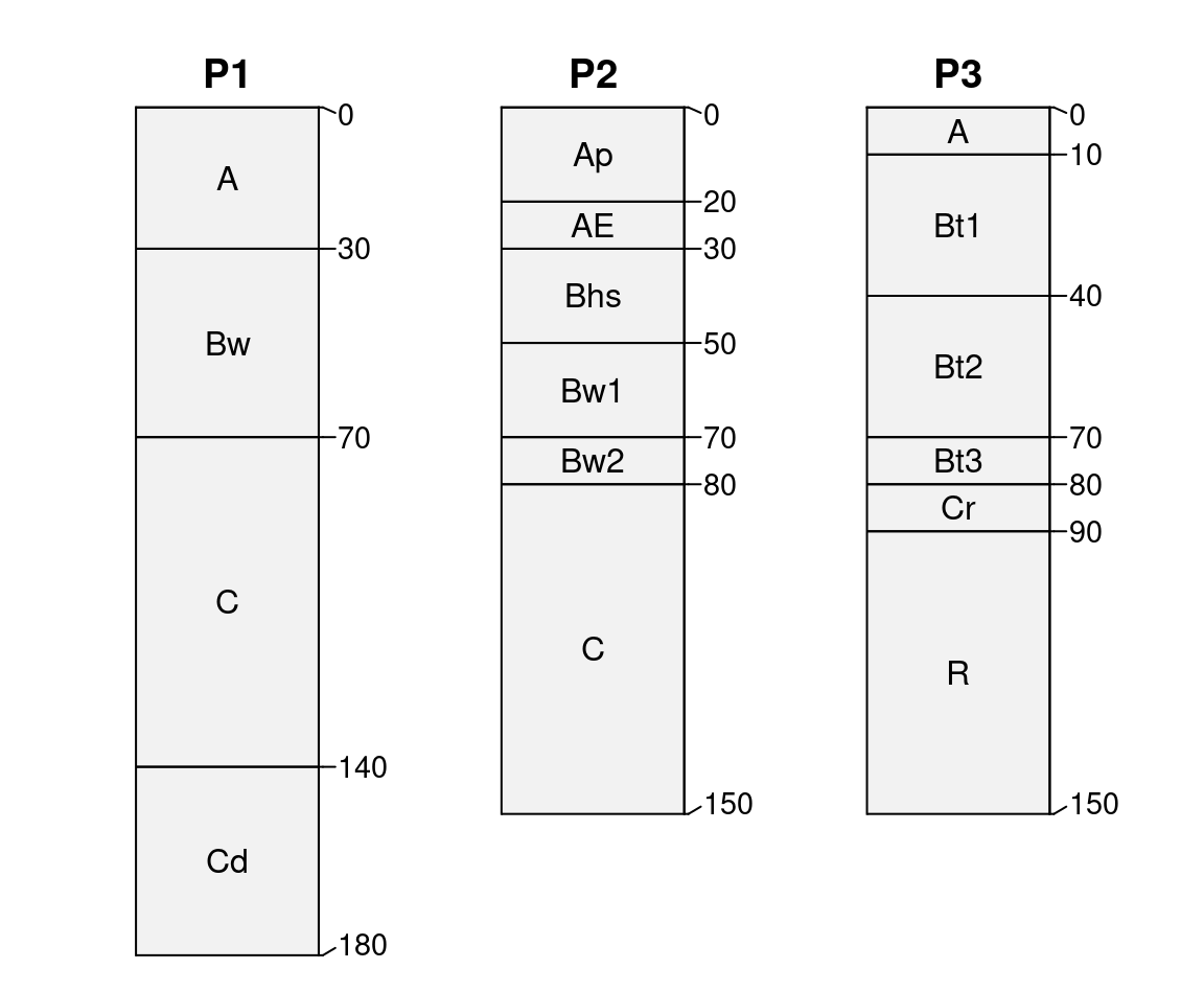
idcolumn ~ hz_top_column + hz_bottom_column

Rapid Templating

Small collections of soil profiles can be described using text “templates” and quickSPC(). Templates take the form of:

• ID:AAA|BBB|CCCCCC: relative thickness specified by horizon designations, split by “|” symbol

• ID:A-B-C: horizons of random thickness specified by horizon designations, split by “-” symbol

The “ID:” prefix is optional, with unique IDs generated by the digest package when omitted.

# character vector of horizon templates
# must all use the same formatting
x <- c(
  'P1:AAA|BwBwBwBw|CCCCCCC|CdCdCdCd',
  'P2:ApAp|AE|BhsBhs|Bw1Bw1|Bw2|CCCCCCC',
  'P3:A|Bt1Bt1Bt1|Bt2Bt2Bt2|Bt3|Cr|RRRRRR'
)

# each horizon label is '10' depth-units (default)
s <- quickSPC(x)

# sketch profiles
par(mar = c(0, 0, 0, 0))
plotSPC(s, name.style = 'center-center', 
        cex.names = 1, depth.axis = FALSE, 
        hz.depths = TRUE
)

Accessing, Setting, and Replacing Data

“Accessor” functions are used to extract specific components from within SoilProfileCollection objects.

• Methods that return a column name. These are useful for extracting depths, horizon designations, IDs, etc. before taking an SPC apart for a specific task.

  • idname(sp4): extract profile ID name (column name used to init SPC)
  • horizonDepths(sp4): horizon top / bottom depth names (used to init SPC)
  • hzidname(sp4): horizon ID name (typically automatically built at init time)
  • hzdesgnname(sp4): horizon designation name (if set)
  • hztexclname(sp4): horizon texture class name (if set)

• Methods that return a vector of values.

  • profile_id(sp4): profile IDs, in order
  • hzID(sp4): horizon IDs, in order
  • hzDesgn(sp4): horizon designations, in order

• Methods that return site/horizon attribute column names.

  • names(sp4): site + horizon names concatenated into a single vector
  • horizonNames(sp4): horizon names
  • siteNames(sp4): site names

• Profile and horizon totals.

  • length(sp4): number of profiles in collection
  • nrow(sp4): number of horizons in collection

• Other methods.

  • depth_units(sp4): defaults to ‘cm’ at SPC creation
  • metadata(sp4): returns list object with base + optional (user-defined) metadata elements

Horizon and Site Data

Horizon data and information about key columns (unique profile ID and depths) are the primary input to the methods provided to create the object. Site data can be derived from unique profile-specific values within the input horizon data, or joined in from an external source based on profile ID.

Both site and horizon data are stored as data.frame within the SoilProfileCollection; with one or more rows (per profile ID) in the horizon table and one row (per profile ID) in the site table. The SoilProfileCollection also supports data.table, or tibble objects in the data.frame slots.

Columns from site or horizon tables can be accessed with the $ syntax notation, similar to the data.frame. New data can be assigned to either table in the same manner, as long as the length of the new data is:

1. same length as the number of profiles in the collection (target is the site table)
2. same length as the number of horizons in the collection (target is the horizon table)
3. length 1; and selecting the target table requires site(object)$new_column <- new_value for new site data and horizons(object)$new_column <- new value for horizon

Assignment of new data to existing or new attributes can proceed as follows.

# site-level (based on length of assigned data == number of profiles)
sp4$elevation <- rnorm(n = length(sp4), mean = 1000, sd = 150) 

# horizon-level (calculated from two horizon-level columns)
sp4$thickness <- sp4$bottom - sp4$top 

# extraction of specific attributes by name
sp4$clay # vector of clay content (horizon data)

#>  [1] 21 27 32 55 25 34  3 15 27 32 25 31 33 13 21 23 15 17 12 19 14 14 22 25 40 51 67 24 25 32

sp4$elevation # vector of simulated elevation (site data)

#>  [1]  789.9935 1038.2976  634.4105  999.1643 1093.2329 1172.2617  726.7274  962.9012  963.3701
#> [10]  957.5942

# unit-length value explicitly targeting site data
site(sp4)$collection_id <- 1

# assign a single single value into horizon-level attributes
sp4$constant <- rep(1, times = nrow(sp4))

# unit-length value explicitly targeting horizon data
horizons(sp4)$analysis_group <- "SERP"

# _moves_ the named column from horizon to site
site(sp4) <- ~ constant 

Horizon and site data can be modified via extraction to data.frame followed by replacement (horizon data) or join (site data). Note that while this approach gives the most flexibility, it is also the most dangerous–replacement of horizon data with new data that don’t exactly conform to the original sorting may corrupt your SoilProfileCollection.

# extract horizon data to data.frame
h <- horizons(sp4)

# add a new column and save back to original object
h$random.numbers <- rnorm(n = nrow(h), mean = 0, sd = 1)

# _replace_ original horizon data with modified version
replaceHorizons(sp4) <- h

# extract site data to data.frame
s <- site(sp4)

# add a fake group to the site data
s$group <- factor(rep(c('A', 'B'), length.out = nrow(s)))

# join new site data with previous data: old data are _not_ replaced
site(sp4) <- s

# check
sp4

#> SoilProfileCollection with 10 profiles and 30 horizons
#> profile ID: id  |  horizon ID: hzID 
#> Depth range: 16 - 49 cm
#> 
#> ----- Horizons (6 / 30 rows  |  10 / 17 columns) -----
#>      id hzID top bottom name   K   Mg  Ca CEC_7 ex_Ca_to_Mg
#>  colusa    1   0      3    A 0.3 25.7 9.0  23.0        0.35
#>  colusa    2   3      8  ABt 0.2 23.7 5.6  21.4        0.23
#>  colusa    3   8     30  Bt1 0.1 23.2 1.9  23.7        0.08
#>  colusa    4  30     42  Bt2 0.1 44.3 0.3  43.0        0.01
#>   glenn    5   0      9    A 0.2 21.9 4.4  18.8        0.20
#>   glenn    6   9     34   Bt 0.3 18.9 4.5  27.5        0.20
#> [... more horizons ...]
#> 
#> ----- Sites (6 / 10 rows  |  5 / 5 columns) -----
#>         id elevation collection_id constant group
#>     colusa  789.9935             1        1     A
#>      glenn 1038.2976             1        1     B
#>      kings  634.4105             1        1     A
#>   mariposa  999.1643             1        1     B
#>  mendocino 1093.2329             1        1     A
#>       napa 1172.2617             1        1     B
#> [... more sites ...]
#> 
#> Spatial Data:
#> [EMPTY]

Diagnostic Horizons

Diagnostic horizons typically span several genetic horizons and may or may not be present in every profile.

To accommodate the wide range of possibilities, diagnostic horizon data are stored as a data.frame in “long format”: each row corresponds to a diagnostic feature in a single profile, identified with a column matching the ID column used to initialize the SoilProfileCollection object and a label reflecting the feature kind.

For diagnostic horizon data there are no restrictions on data content, as long as each row has an ID that exists within the collection. Be sure to use the ID column name that was used to initialize the SoilProfileCollection object.

dh <- data.frame(
  id = 'colusa',
  kind = 'argillic',
  top = 8,
  bottom = 42,
  stringsAsFactors = FALSE
)

# overwrite any existing diagnostic horizon data
diagnostic_hz(sp4) <- dh

# append to diagnostic horizon data
dh <- diagnostic_hz(sp4)
dh.new <- data.frame(
  id = 'napa',
  kind = 'argillic',
  top = 6,
  bottom = 20,
  stringsAsFactors = FALSE
)

# overwrite existing diagnostic horizon data with appended data
diagnostic_hz(sp4) <- rbind(dh, dh.new)

Root Restrictive Features

Features that restrict root entry (fine or very fine roots) are commonly used to estimate functional soil depth. Restrictive features include salt accumulations, duripans, fragipans, paralithic materials, lithic contact, or an abrupt change in chemical property.

Not all soils have restrictive features, therefore these data are stored as a data.frame in “long format”. Each row corresponds to a restrictive feature, associated depths, and identified by profile_id(). There may be more than one restrictive feature per soil profile.

The example data sp4 does not describe the restrictive features, so we will simulate some at the bottom of each profile + 20cm.

# get the depth of each profile
rf.top <- profileApply(sp4, max)
rf.bottom <- rf.top + 20

# the profile IDs can be extracted from the names attribute
pIDs <- names(rf.top)

# note: profile IDs must be stored in a column named for idname(sp4) -> 'id'
rf <- data.frame(
  id = pIDs, 
  top = rf.top, 
  bottom = rf.bottom, 
  kind = 'fake',
  stringsAsFactors = FALSE
)

# overwrite any existing diagnostic horizon data
restrictions(sp4) <- rf

# check
restrictions(sp4)

#>                id top bottom kind
#> 1          colusa  42     62 fake
#> 2           glenn  34     54 fake
#> 3           kings  40     60 fake
#> 4        mariposa  49     69 fake
#> 5       mendocino  30     50 fake
#> 6            napa  20     40 fake
#> 7      san benito  20     40 fake
#> 8          shasta  40     60 fake
#> 9  shasta-trinity  40     60 fake
#> 10         tehama  16     36 fake

Object Metadata

SoilProfileCollection metadata can be extracted and set using the metadata() and metadata<- methods.

# metadata structure
str(metadata(sp4))

#> List of 6
#>  $ aqp_df_class    : chr "data.frame"
#>  $ aqp_group_by    : chr ""
#>  $ aqp_hzdesgn     : chr "name"
#>  $ aqp_hztexcl     : chr ""
#>  $ depth_units     : chr "cm"
#>  $ stringsAsFactors: logi FALSE

# alter the depth unit metadata attribute
depth_units(sp4) <- 'inches' # units are really 'cm'

# add or replace custom metadata
metadata(sp4)$describer <- 'DGM'
metadata(sp4)$date <- as.Date('2009-01-01')
metadata(sp4)$citation <- 'McGahan, D.G., Southard, R.J, Claassen, V.P. 2009. Plant-Available Calcium Varies Widely in Soils on Serpentinite Landscapes. Soil Sci. Soc. Am. J. 73: 2087-2095.'

# check new values have been added
str(metadata(sp4))

#> List of 9
#>  $ aqp_df_class    : chr "data.frame"
#>  $ aqp_group_by    : chr ""
#>  $ aqp_hzdesgn     : chr "name"
#>  $ aqp_hztexcl     : chr ""
#>  $ depth_units     : chr "inches"
#>  $ stringsAsFactors: logi FALSE
#>  $ describer       : chr "DGM"
#>  $ date            : Date[1:1], format: "2009-01-01"
#>  $ citation        : chr "McGahan, D.G., Southard, R.J, Claassen, V.P. 2009. Plant-Available Calcium Varies Widely in Soils on Serpentini"| __truncated__

# fix depth units, set back to 'cm'
depth_units(sp4) <- 'cm'

Spatial Data

Spatial data and metadata can be stored within a SoilProfileCollection object. To initialize a “spatial” SoilProfileCollection, use initSpatial()<- method. This allows you to specify which columns contain the geometry and optionally the Coordinate Reference System of those data. The SoilProfileCollection stores two metadata entries: coordinates and crs which refer to the column names containing geometric data and the CRS, respectively.

# generate some fake coordinates as site level attributes
sp4$x <- rnorm(n = length(sp4), mean = 354000, sd = 100)
sp4$y <- rnorm(n = length(sp4), mean = 4109533, sd = 100)

# initialize spatial coordinates (CRS optional)
initSpatial(sp4, crs = "EPSG:26911") <- ~ x + y

# extract coordinates as matrix
getSpatial(sp4)

#>              x       y
#>  [1,] 354007.0 4109619
#>  [2,] 353936.1 4109509
#>  [3,] 353995.0 4109512
#>  [4,] 353974.9 4109535
#>  [5,] 354044.5 4109536
#>  [6,] 354275.5 4109588
#>  [7,] 354004.7 4109306
#>  [8,] 354057.8 4109801
#>  [9,] 354011.8 4109497
#> [10,] 353808.8 4109554

# get/set spatial reference system using prj()<-
prj(sp4) <- '+proj=utm +zone=11 +datum=NAD83'

# return CRS information
prj(sp4)

#> [1] "+proj=utm +zone=11 +datum=NAD83"

# extract spatial data + site level attributes in new spatial object
sp4.sp <- as(sp4, 'SpatialPointsDataFrame')
sp4.sf <- as(sp4, 'sf')

Validity and Horizon Logic

There are several SoilProfileCollection methods defined to identify corrupted objects/bad depth logic and fix them.

Usually an “invalid” or “corrupt” SoilProfileCollection comes from direct modification of the S4 object slot contents (not using standard methods), which can result in omissions or reordering that bypasses internal accounting methods.

Occasionally issues arise from illogical inputs (depths) or collections that are missing data. The latter cases (standard methods produce a corrupt SPC given some “degenerate” input data) are considered “bugs” that should reported on the issue tracker: https://github.com/ncss-tech/aqp/issues

checkSPC() returns TRUE for a SoilProfileCollection that contains all slots defined in the class prototype.

checkSPC(sp4)

spc_in_sync() is used as the validity method for the SoilProfileCollection, it determines if some reordering of the horizon data relative to the unique profile ID / site order has occurred.

spc_in_sync(sp4)

#>   nSites relativeOrder valid
#> 1   TRUE          TRUE  TRUE

rebuildSPC() is used to re-construct all the required slots of a SoilProfileCollection, given a source, possibly corrupt, object. This function fixes major issues related to the internal ordering of data in slots, as well as missing slots or metadata.

z <- rebuildSPC(sp4)

checkHzDepthLogic() has the ability to perform logical tests on whole profiles or individual horizons. Four different tests are performed related to four common errors in horizon depths:

• bottom depth shallower than top depth

• equal top and bottom depth

• missing (NA) top or bottom depth

• gap or overlap between adjacent horizons

checkHzDepthLogic(sp4)

#>                id valid depthLogic sameDepth missingDepth overlapOrGap
#> 1          colusa  TRUE      FALSE     FALSE        FALSE        FALSE
#> 2           glenn  TRUE      FALSE     FALSE        FALSE        FALSE
#> 3           kings  TRUE      FALSE     FALSE        FALSE        FALSE
#> 4        mariposa  TRUE      FALSE     FALSE        FALSE        FALSE
#> 5       mendocino  TRUE      FALSE     FALSE        FALSE        FALSE
#> 6            napa  TRUE      FALSE     FALSE        FALSE        FALSE
#> 7      san benito  TRUE      FALSE     FALSE        FALSE        FALSE
#> 8          shasta  TRUE      FALSE     FALSE        FALSE        FALSE
#> 9  shasta-trinity  TRUE      FALSE     FALSE        FALSE        FALSE
#> 10         tehama  TRUE      FALSE     FALSE        FALSE        FALSE

checkHzDepthLogic(sp4, byhz = TRUE)

#>                id top bottom valid hzID depthLogic sameDepth missingDepth overlapOrGap
#> 1          colusa   0      3  TRUE    1      FALSE     FALSE        FALSE           NA
#> 2          colusa   3      8  TRUE    2      FALSE     FALSE        FALSE           NA
#> 3          colusa   8     30  TRUE    3      FALSE     FALSE        FALSE           NA
#> 4          colusa  30     42  TRUE    4      FALSE     FALSE        FALSE           NA
#> 5           glenn   0      9  TRUE    5      FALSE     FALSE        FALSE           NA
#> 6           glenn   9     34  TRUE    6      FALSE     FALSE        FALSE           NA
#> 7           kings   0      4  TRUE    7      FALSE     FALSE        FALSE           NA
#> 8           kings   4     13  TRUE    8      FALSE     FALSE        FALSE           NA
#> 9           kings  13     40  TRUE    9      FALSE     FALSE        FALSE           NA
#> 10       mariposa   0      3  TRUE   10      FALSE     FALSE        FALSE           NA
#> 11       mariposa   3     14  TRUE   11      FALSE     FALSE        FALSE           NA
#> 12       mariposa  14     34  TRUE   12      FALSE     FALSE        FALSE           NA
#> 13       mariposa  34     49  TRUE   13      FALSE     FALSE        FALSE           NA
#> 14      mendocino   0      2  TRUE   14      FALSE     FALSE        FALSE           NA
#> 15      mendocino   2      8  TRUE   15      FALSE     FALSE        FALSE           NA
#> 16      mendocino   8     30  TRUE   16      FALSE     FALSE        FALSE           NA
#> 17           napa   0      6  TRUE   17      FALSE     FALSE        FALSE           NA
#> 18           napa   6     20  TRUE   18      FALSE     FALSE        FALSE           NA
#> 19     san benito   0      8  TRUE   19      FALSE     FALSE        FALSE           NA
#> 20     san benito   8     20  TRUE   20      FALSE     FALSE        FALSE           NA
#> 21         shasta   0      3  TRUE   21      FALSE     FALSE        FALSE           NA
#> 22         shasta   3     40  TRUE   22      FALSE     FALSE        FALSE           NA
#> 23 shasta-trinity   0      2  TRUE   23      FALSE     FALSE        FALSE           NA
#> 24 shasta-trinity   2      5  TRUE   24      FALSE     FALSE        FALSE           NA
#> 25 shasta-trinity   5     12  TRUE   25      FALSE     FALSE        FALSE           NA
#> 26 shasta-trinity  12     23  TRUE   26      FALSE     FALSE        FALSE           NA
#> 27 shasta-trinity  23     40  TRUE   27      FALSE     FALSE        FALSE           NA
#> 28         tehama   0      3  TRUE   28      FALSE     FALSE        FALSE           NA
#> 29         tehama   3      7  TRUE   29      FALSE     FALSE        FALSE           NA
#> 30         tehama   7     16  TRUE   30      FALSE     FALSE        FALSE           NA

Coercion

SoilProfileCollection objects can be coerced to data.frame, list and SpatialPointsDataFrame (when spatial slot has been set up):

# check our work by viewing the internal structure
str(sp4)

# create a data.frame from horizon+site data
as(sp4, 'data.frame') 

# or, equivalently:
as.data.frame(sp4)

# convert SoilProfileCollection to a named list containing all slots
as(sp4, 'list')

# extraction of site + spatial data as SpatialPointsDataFrame
as(sp4, 'SpatialPointsDataFrame')

Subsetting SoilProfileCollection Objects

SoilProfileCollection objects can be subset using the familiar [-style notation used by matrix and data.frame objects, such that: spc[i, j] will return profiles identified by the integer vector i, and horizons identified by the integer vector j.

Omitting either index will result in all profiles (i omitted) or all horizons (j omitted).

Typically, site-level attributes will be used as the subsetting criteria. Functions that return an index to matches (such as grep() or which()) provide the link between attributes and an index to matching profiles.

Profiles

Using the i index, select one or more profiles by numeric index. An index greater than the number of profiles will return an empty SoilProfileCollection object.

# explicit string matching
idx <- which(sp4$group == 'A')

# numerical expressions
idx <- which(sp4$elevation < 1000)

# regular expression, matches any profile ID containing 'shasta'
idx <- grep('shasta', profile_id(sp4), ignore.case = TRUE)

# perform subset based on index
sp4[idx, ]

In an interactive session, it is often simpler to use subset() directly:

subset(sp4, group == 'A')
subset(sp4, elevation < 1000)
subset(sp4, grepl('shasta', id, ignore.case = TRUE))

Horizons by Index

Using the j index, select the 2nd horizon from each profile in the collection. Use with caution, asking for a horizon beyond the length of any profile in the collection will result in an error.

sp4[, 2]

Horizons by Keyword

Using the k index, select the .FIRST first or .LAST horizons (by profile) within a collection. Note that .FIRST and .LAST are special keywords used by the SoilProfileCollection subset methods.

sp4[, , .FIRST]
sp4[, , .LAST]

Splitting, Duplication, and Selection of Unique Profiles

SoilProfileCollection objects are combined by passing a list of objects to the combine() function.

Ideally all objects share the same internal structure, profile ID, horizon ID, depth units, and other parameters of a SoilProfileCollection. Manually subset the example data into 3 pieces, compile into a list, and then combine back together.

# subset data into chunks
s1 <- sp4[1:2, ]
s2 <- sp4[4, ]
s3 <- sp4[c(6, 8, 9), ]

# combine subsets
s <- combine(list(s1, s2, s3))

# double-check result
plotSPC(s)

It is possible to combine SoilProfileCollection objects with different internal structure. The final object will contain the all site and horizon columns from the inputs, possibly creating sparse tables. IDs and horizon depth names are taken from the first object.

# sample data as data.frame objects
data(sp1)
data(sp3)

# rename IDs horizon top / bottom columns
sp3$newid <- sp3$id
sp3$hztop <- sp3$top
sp3$hzbottom <- sp3$bottom

# remove originals
sp3$id <- NULL
sp3$top <- NULL
sp3$bottom <- NULL

# promote to SoilProfileCollection
depths(sp1) <- id ~ top + bottom
depths(sp3) <- newid ~ hztop + hzbottom

# label each group via site-level attribute
site(sp1)$g <- 'sp1'
site(sp3)$g <- 'sp3'

# combine
x <- combine(list(sp1, sp3))

# make grouping variable into a factor for groupedProfilePlot
x$g <- factor(x$g)

# check results
str(x)

# graphical check
# convert character horizon IDs into numeric
x$.horizon_ids_numeric <- as.numeric(hzID(x))

par(mar = c(0, 0, 3, 1))
plotSPC(x, color='.horizon_ids_numeric', col.label = 'Horizon ID')
groupedProfilePlot(x, 'g', color='.horizon_ids_numeric', col.label = 'Horizon ID', group.name.offset = -15)

Splitting

The inverse of combine() is split(): subsets of the SoilProfileCollection are split into list elements, each containing a new SoilProfileCollection.

# continuing from above
# split subsets of x into a list of SoilProfileCollection objects using site-level attribute 'g'
res <- split(x, 'g')
str(res, 1)

Duplication

Duplicate the first profile in sp4 (Colusa) 8 times, resulting in a new SoilProfileCollection object containing unique profile IDs.

d <- duplicate(sp4[1, ], times = 8)
par(mar = c(0, 2, 0, 1))
plotSPC(d, color = 'ex_Ca_to_Mg')

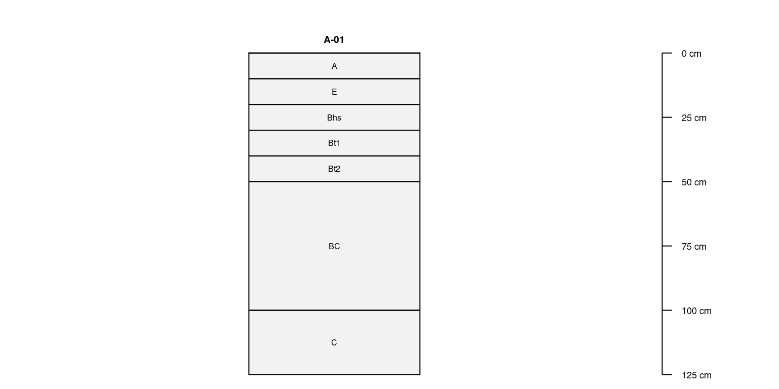
Selecting Unique Profiles

# an example soil profile  
x <- data.frame(
  id = 'A',
  name = c('A', 'E', 'Bhs', 'Bt1', 'Bt2', 'BC', 'C'),
  top = c(0, 10, 20, 30, 40, 50, 100),
  bottom = c(10, 20, 30, 40, 50, 100, 125),
  z = c(8, 5, 3, 7, 10, 2, 12)
)

# init SPC
depths(x) <- id ~ top + bottom
hzdesgnname(x) <- 'name'

# horizon depth variability for simulation
horizons(x)$.sd <- 2

# duplicate several times
x.dupes <- duplicate(x, times = 5)

# simulate some new profiles based on example
# 2cm constant standard deviation of transition between horizons assumed
x.sim <- perturb(x, n = 5, thickness.attr = '.sd')

# graphical check
par(mar = c(0, 2, 0, 4))

# inspect unique results
plotSPC(unique(x.dupes, vars = c('top', 'bottom')),
        name.style = 'center-center',
        width = 0.15)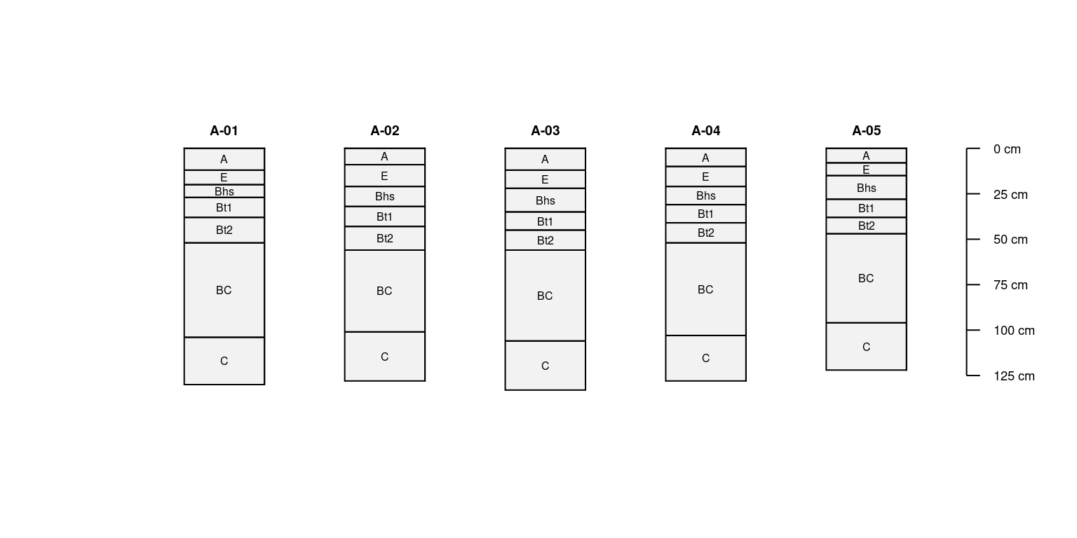

# "uniqueness" is a function of variables selected to consider
plotSPC(unique(x.sim, vars = c('top', 'bottom')),
        name.style = 'center-center')

plotSPC(unique(x.sim, vars = c('name')),
        name.style = 'center-center',
        width = 0.15)

Plotting SoilProfileCollection Objects

The plotSPC() method for SoilProfileCollection objects generates sketches of profiles within the collection based on horizon boundaries, vertically aligned to an integer sequence from 1 to the number of profiles.

Horizon names are automatically extracted from a horizon-level attribute name (if present), or via an alternate attributed given as an argument: name='column.name'.

Horizon colors are automatically generated from the horizon-level attribute soil_color, or any other attribute of R-compatible color description given as an argument: color='column.name'. This function is highly customizable, therefore, it is prudent to consult help(plotSPC) from time to time. Soil colors in Munsell notation can be converted to R-compatible colors via munsell2rgb().

Many of the following examples make use of par() to set graphical options such as mar (customized margins) and/or xpd = NA (turn off clipping) to optimize display of different numbers of profiles and various plotSPC() arguments.

A detailed description of each argument to plotSPC() (and many examples) can be found in the Soil Profile Sketches tutorial.

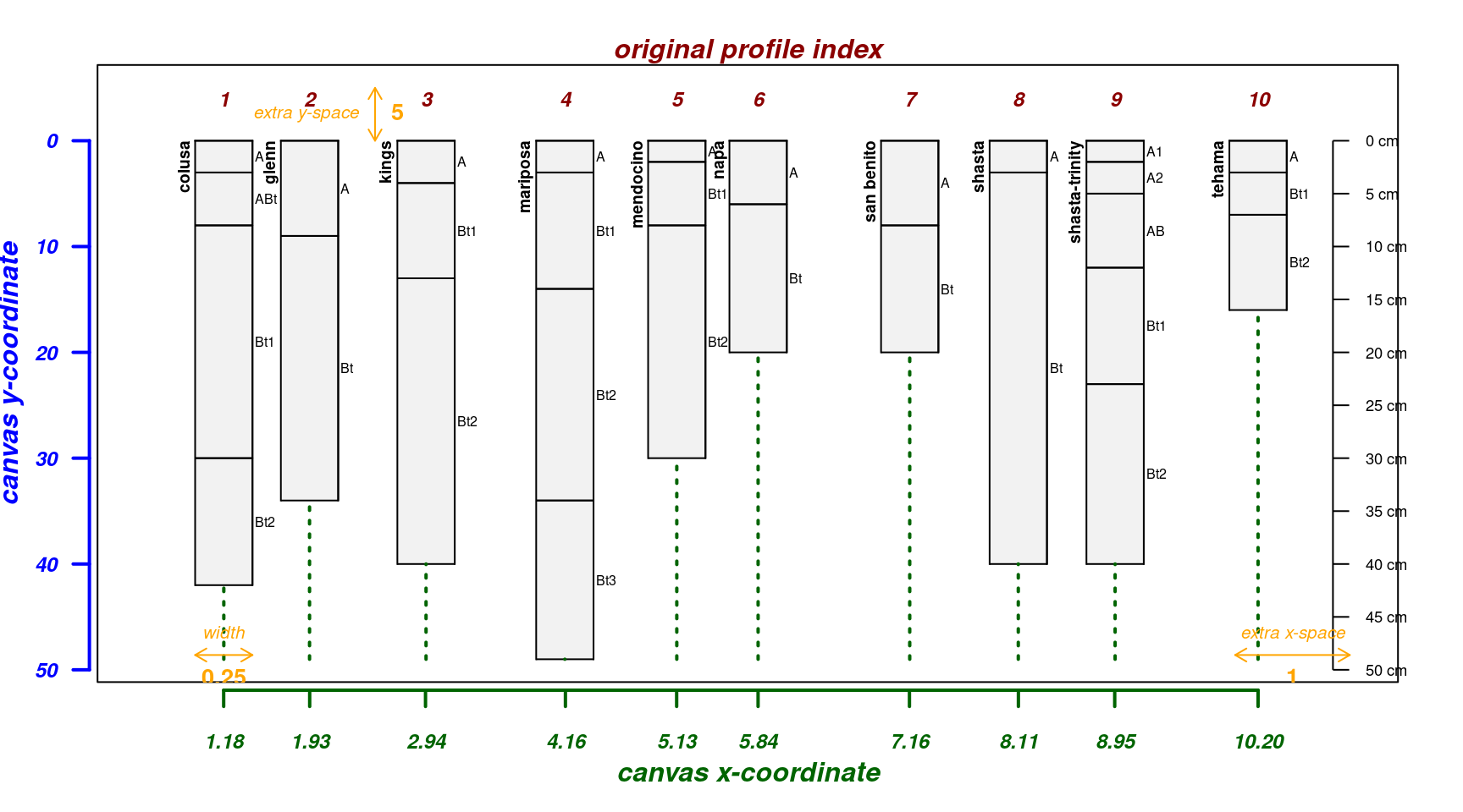
Making Adjustments

The explainPlotSPC() function is helpful for adjusting some of the more obscure arguments to plotSPC().

A basic plot with debugging information overlaid:

par(mar = c(4, 3, 2, 2))
explainPlotSPC(sp4, name = 'name')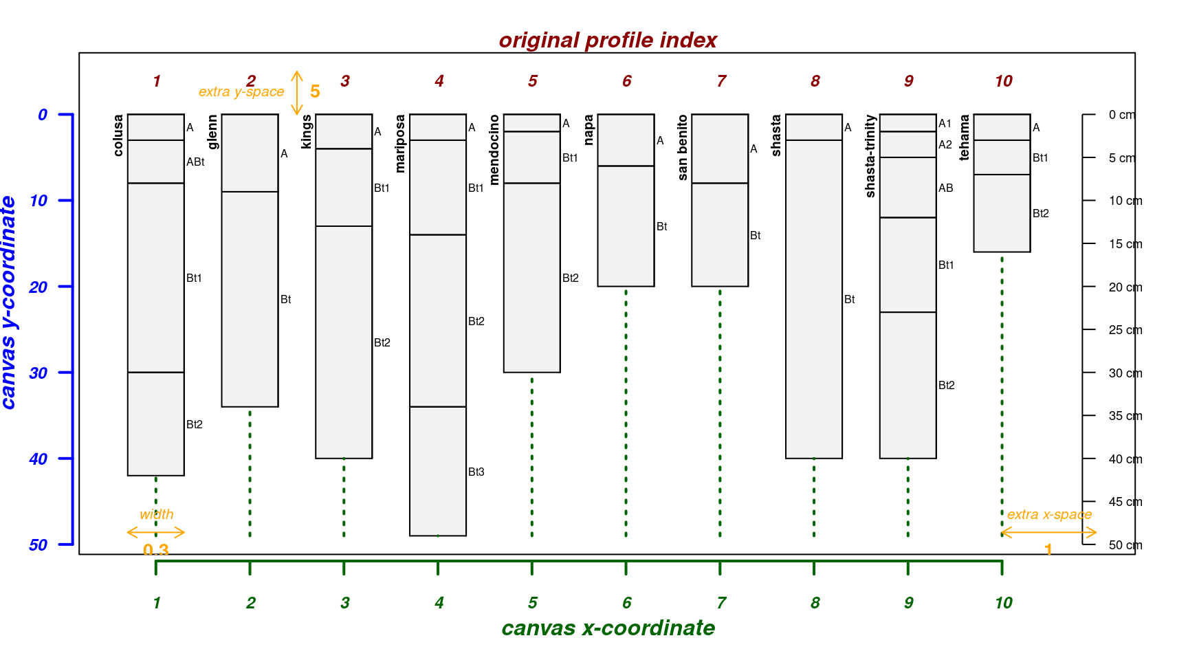

Make sketches wider:

par(mar = c(4, 3, 2, 2))
explainPlotSPC(sp4, name = 'name', width = 0.3)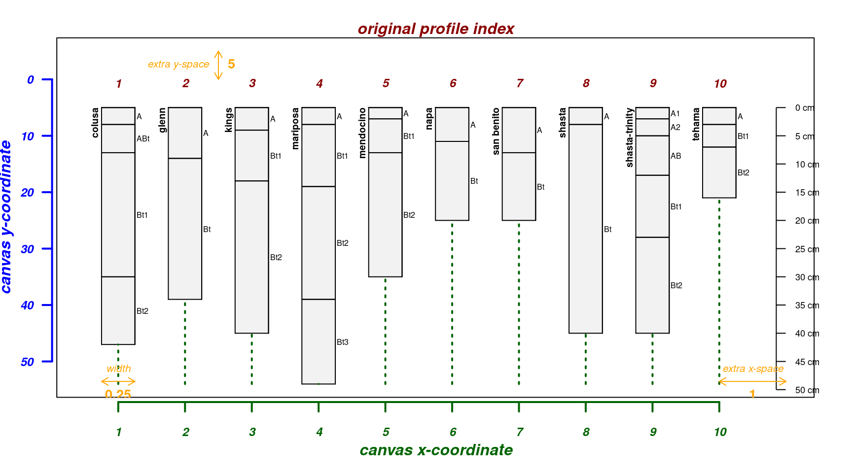

Move soil surface at 0cm “down” 5cm:

par(mar = c(4, 3, 2, 2))
explainPlotSPC(sp4, name = 'name', y.offset = 5)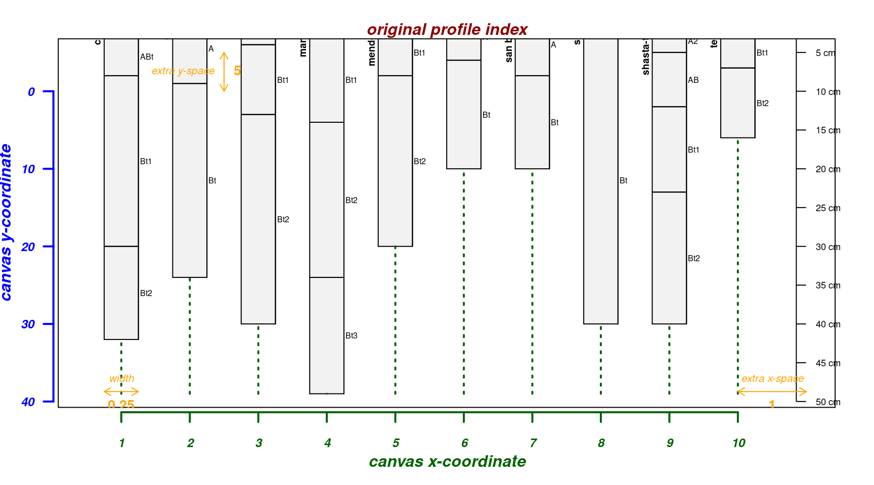

Move soil surface at 0cm “up” 10cm; useful for sketches of shallow profiles:

par(mar = c(4, 3, 2, 2))
explainPlotSPC(sp4, name = 'name', y.offset = -10)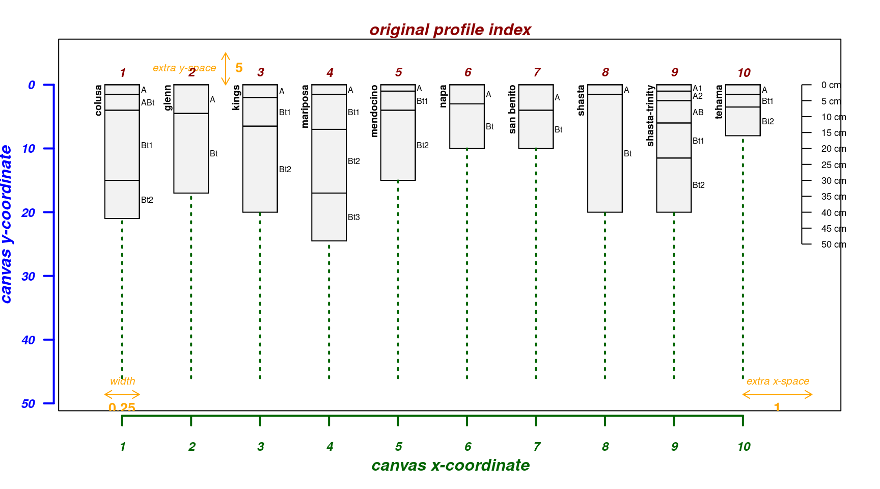

Scale depths by 50%:

par(mar = c(4, 3, 2, 2))
explainPlotSPC(sp4, name = 'name', scaling.factor = 0.5)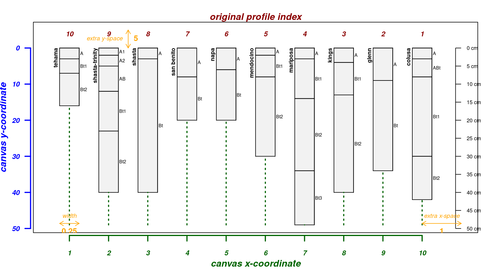

A graphical explanation of how profiles are re-arranged via plot.order argument:

par(mar = c(4, 3, 2, 2))
explainPlotSPC(sp4, name = 'name', plot.order = length(sp4):1)

Leave room for an additional 2 profile sketches:

par(mar = c(4, 3, 2, 2))
explainPlotSPC(sp4, name = 'name', n = length(sp4) + 2)

Small SoilProfileCollections

Making quality figures with fewer than 5 soil profiles usually requires more customization of the basic call to plotSPC. In general, the following are a good starting point:

• shrink margins and disable clipping with par
• adjust output graphic device (e.g. png()) dimensions and resolution
• increase font size with cex.names
• adjust sketch width with width, typically within 0.15-0.35
• move depth axis to the left using negative line values, e.g. (depth.axis = list(line = -2))

Get some example data from the Official Series Descriptions:

data(osd)
x <- osd

Using 5x6 inch output device:

par(mar = c(0, 2, 0, 4), xpd = NA)
plotSPC(x[1, ], cex.names = 1)

Using 7x6 inch output device, slight adjustments to width usually required:

# set margins and turn off clipping
par(mar = c(0, 2, 0, 4), xpd = NA)
plotSPC(x[1:2, ], cex.names = 1, width = 0.25)

Using 8x6 inch output device, slight adjustments to are usually required:

par(mar = c(0, 2, 0, 4), xpd = NA)
plotSPC(x, cex.names = 1, depth.axis = list(line = -0.1), width = 0.3)

Horizon Depth Labeling

Horizon depths can be labeled for each profile as an alternative to a single depth axis.

par(mar = c(0, 0, 1, 1))
plotSPC(
  x,
  cex.names = 1,
  name.style = 'center-center',
  width = 0.3,
  depth.axis = FALSE,
  hz.depths = TRUE,
  hz.depths.offset = 0.08
)

As of aqp version 1.41, it is possible to “fix” overlapping horizon depth labels with the new fixLabelCollisions argument. This approach to labeling depths works best when moving horizon designations with the name.style argument. Note that setting fixLabelCollisions = TRUE may incur a performance penalty when plotting large SoilProfileCollection objects.

As of aqp version 2.0, fixLabelCollisions is set to TRUE when setting hz.depths = TRUE.

Relative Horizontal Positioning

Relative horizontal positioning via relative.pos argument. Can be used with plot.order but be careful: relative.pos must be specified in the final ordering of profiles. See ?plotSPC for details.

par(mar = c(4, 3, 2, 2))
pos <- jitter(1:length(sp4))
explainPlotSPC(sp4, name = 'name', relative.pos = pos)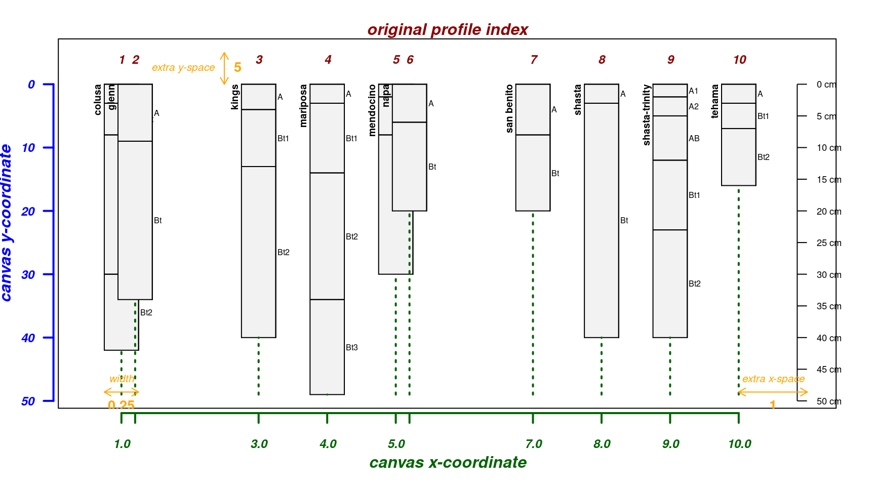

Relative positioning works well when the vector of positions is close to the default spacing along an integer sequence, but not when positions are closer than the width of a profile sketch.

par(mar = c(4, 3, 2, 2))
pos <- c(1, 1.2, 3, 4, 5, 5.2, 7, 8, 9, 10)
explainPlotSPC(sp4, name = 'name', relative.pos = pos)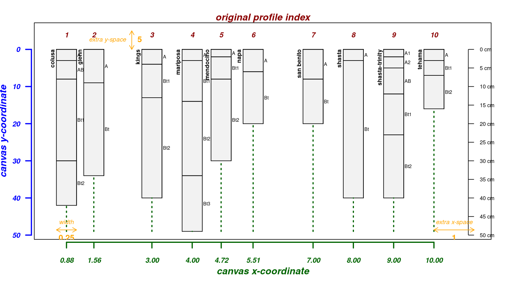

The fixOverlap() function can be used to find a suitable arrangement of profiles based on a compromise between the suggested relative positions and minimization of overlap.

This is an iterative procedure, based on random perturbations of overlapping profiles, therefore it is possible for the algorithm to stop at a sub-optimal configuration. Results can be controlled using set.seed().

par(mar = c(4, 3, 2, 2))
new.pos <- fixOverlap(pos)
explainPlotSPC(sp4, name = 'name', relative.pos = new.pos)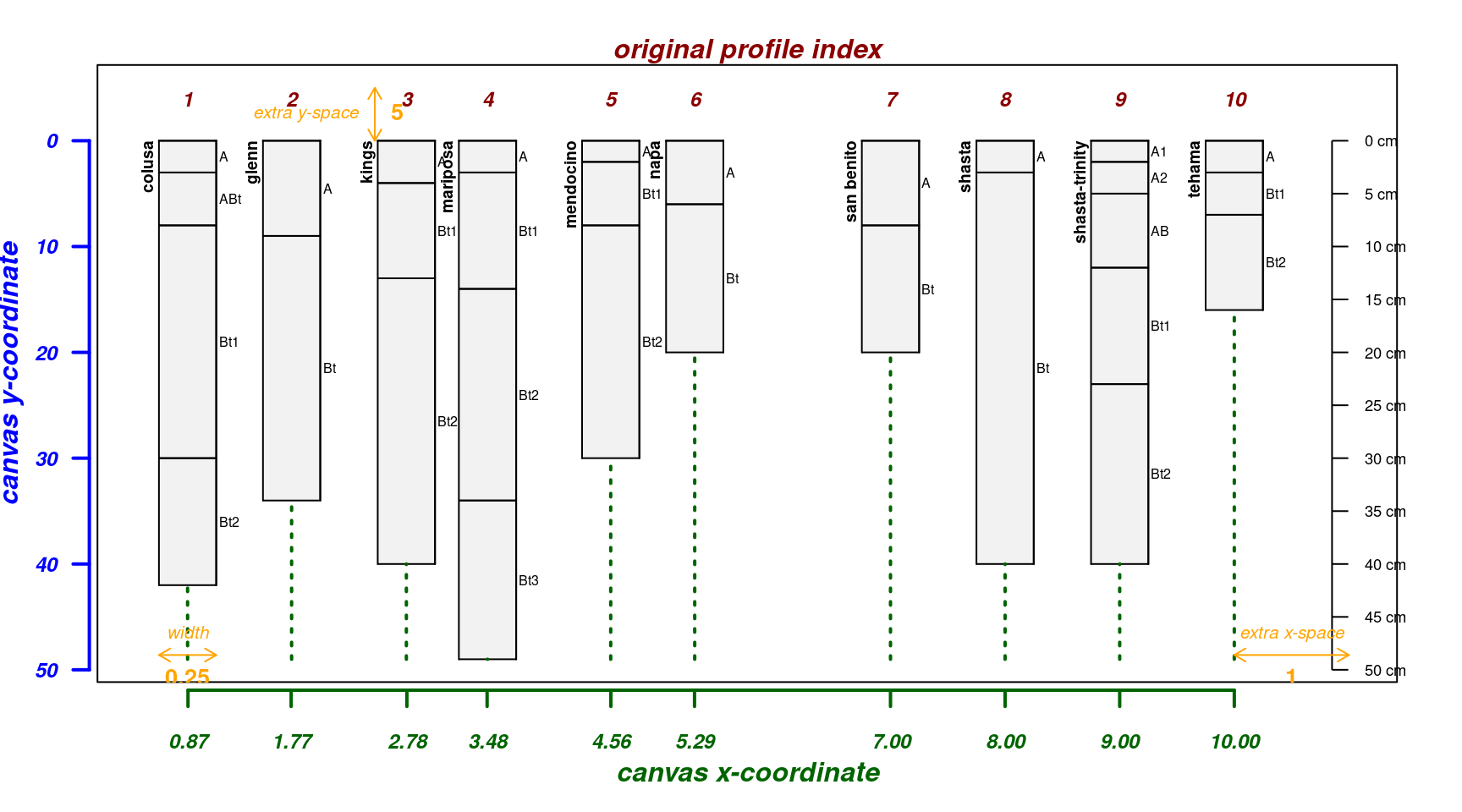

There are several parameters available for optimizing horizontal position in the presence of overlap. See ?fixOverlap for details and further examples.

par(mar = c(4, 3, 2, 2))
new.pos <- fixOverlap(pos, thresh = 0.7)
explainPlotSPC(sp4, name = 'name', relative.pos = new.pos)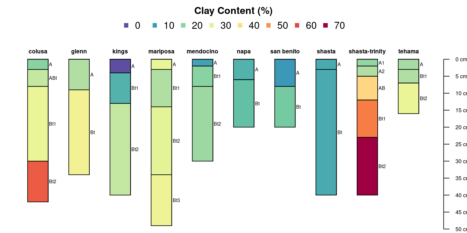

The SPC plotting ideas tutorial contains several additional examples.

Thematic Sketches

Horizon-level attributes can be symbolized with color, in this case using the horizon-level attribute “clay”:

par(mar = c(0, 0, 3, 0))
plotSPC(sp4,
        name = 'name',
        color = 'clay',
        col.label = 'Clay Content (%)')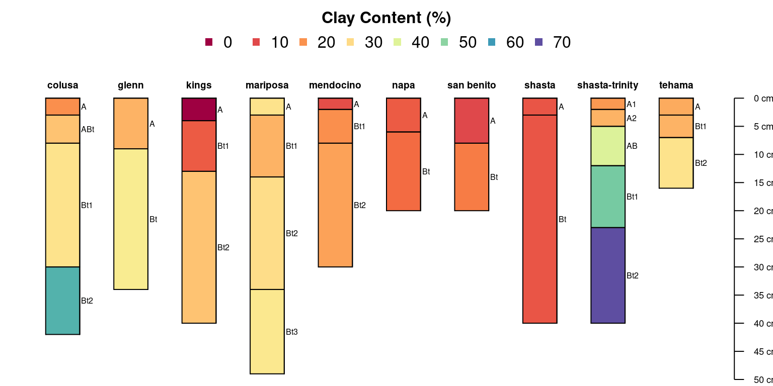

Use a different set of colors:

par(mar = c(0, 0, 3, 0)) 
plotSPC(
  sp4,
  name = 'name',
  color = 'clay',
  col.palette = RColorBrewer::brewer.pal(10, 'Spectral'),
  col.label = 'Clay Content (%)'
)

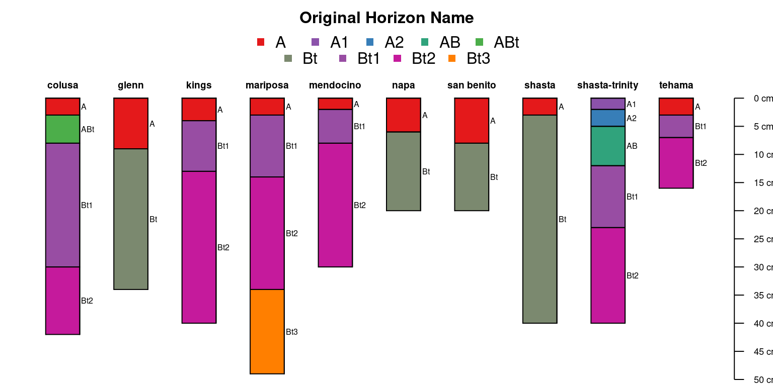
Categorical properties can also be used to make a thematic sketch. Colors are interpolated when there are more classes than colors provided by col.palette:

par(mar = c(0, 0, 3, 0))
plotSPC(
  sp4,
  name = 'name',
  color = 'name',
  col.palette = RColorBrewer::brewer.pal(5, 'Set1'),
  col.label = 'Original Horizon Name'
)

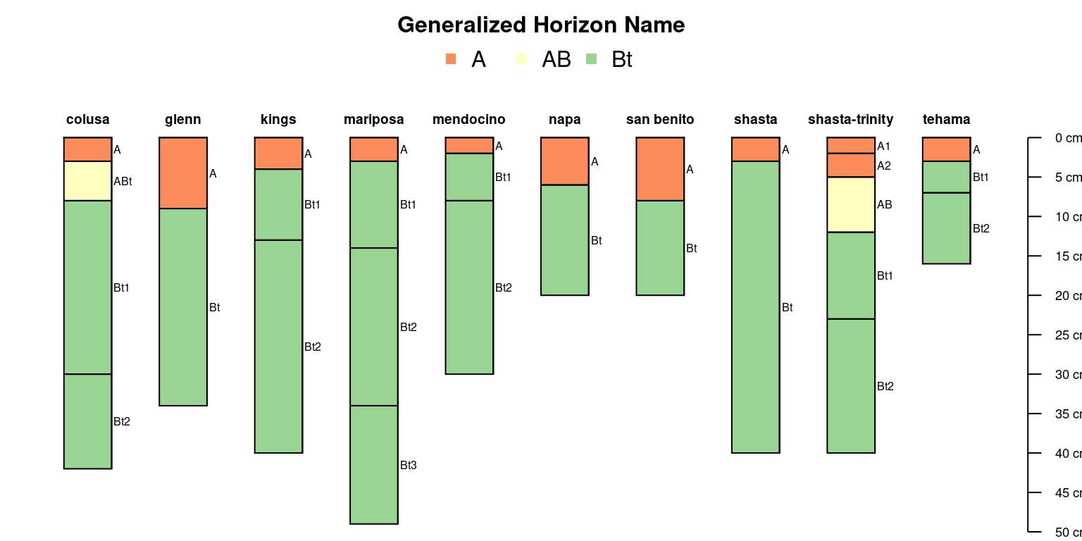
Try with generalized horizon labels:

par(mar = c(0, 0, 3, 0)) 

# generalize horizon names into 3 groups
sp4$genhz <- generalize.hz(sp4$name, new = c('A', 'AB', 'Bt'), pat = c('A[0-9]?', 'AB', '^Bt'))

plotSPC(
  sp4,
  name = 'name',
  color = 'genhz',
  col.palette = RColorBrewer::brewer.pal(3, 'Spectral'),
  col.label = 'Generalized Horizon Name'
)

Horizon-level attributes that represent a volume fraction (e.g. coarse-fragment percentage) can be added to an existing figure. See ?addVolumeFraction for adding layers to an existing plot based on these attributes.

par(mar = c(0, 0, 3, 0)) 
# convert coarse rock fragment proportion to percentage
sp4$frag_pct <- sp4$CF * 100

# label horizons with fragment percent
plotSPC(sp4, name = 'frag_pct', color = 'frag_pct')

# symbolize volume fraction data
addVolumeFraction(sp4, colname = 'frag_pct')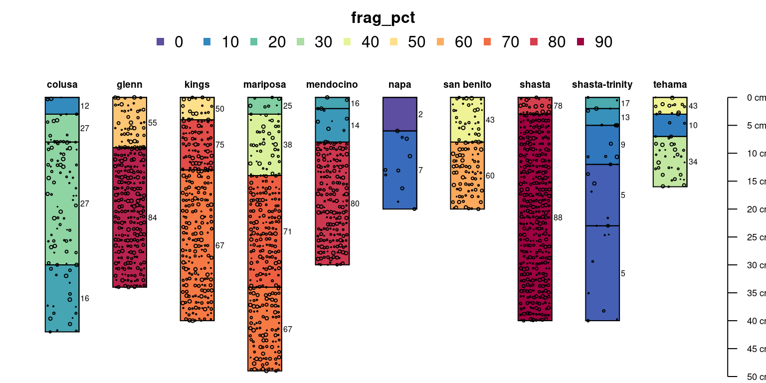

Depth Intervals

Annotation of depth-intervals can be accomplished using “brackets”. Here we extract top/bottom depths associated with top and bottom depth A horizons using the min/max variants of the depthOf() function. See ?depthOf for more details.

# extract top/bottom depths associated with all A horizons
tops <- minDepthOf(sp4, pattern = '^A', hzdesgn = 'name', top = TRUE)
bottoms <- maxDepthOf(sp4, pattern = '^A', hzdesgn = 'name', top = FALSE)

IDs <- profile_id(sp4)

# assemble data.frame
a <- data.frame(id = IDs, top = tops$top, bottom = bottoms$bottom)

# check
a

#>                id top bottom
#> 1          colusa   0      8
#> 2           glenn   0      9
#> 3           kings   0      4
#> 4        mariposa   0      3
#> 5       mendocino   0      2
#> 6            napa   0      6
#> 7      san benito   0      8
#> 8          shasta   0      3
#> 9  shasta-trinity   0     12
#> 10         tehama   0      3

par(mar = c(0, 0, 0, 0))
plotSPC(sp4)

# annotate A horizon depth interval with brackets
addBracket(a, col = 'red', offset = -0.4)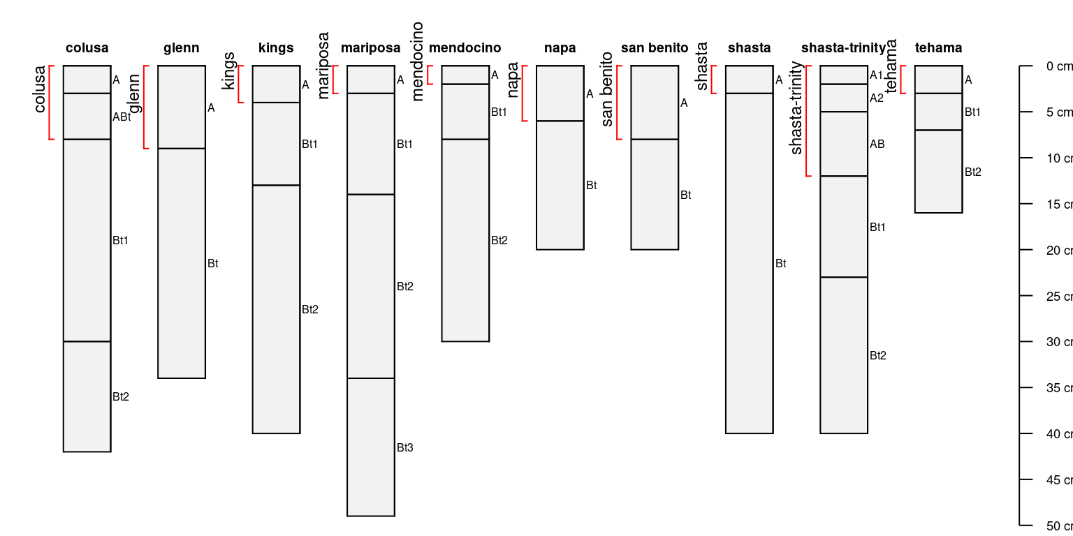

Add labels:

par(mar = c(0, 0, 0, 0))
plotSPC(sp4, name = 'name')

# addBracket() looks for a column `label`; add a ID for each bracket
a$label <- site(sp4)$id

# note that depth brackets "knows which profiles to use" via profile ID
addBracket(
  a,
  col = 'red',
  label.cex = 0.75,
  missing.bottom.depth = 25,
  offset = -0.4
)

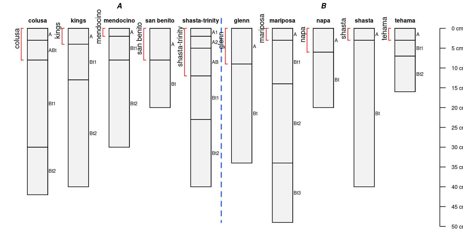
It is possible to arrange profile sketches by site-level grouping variable:

par(mar = c(0, 0, 0, 0)) 
groupedProfilePlot(sp4, groups = 'group')
addBracket(a, col = 'red', offset = -0.4)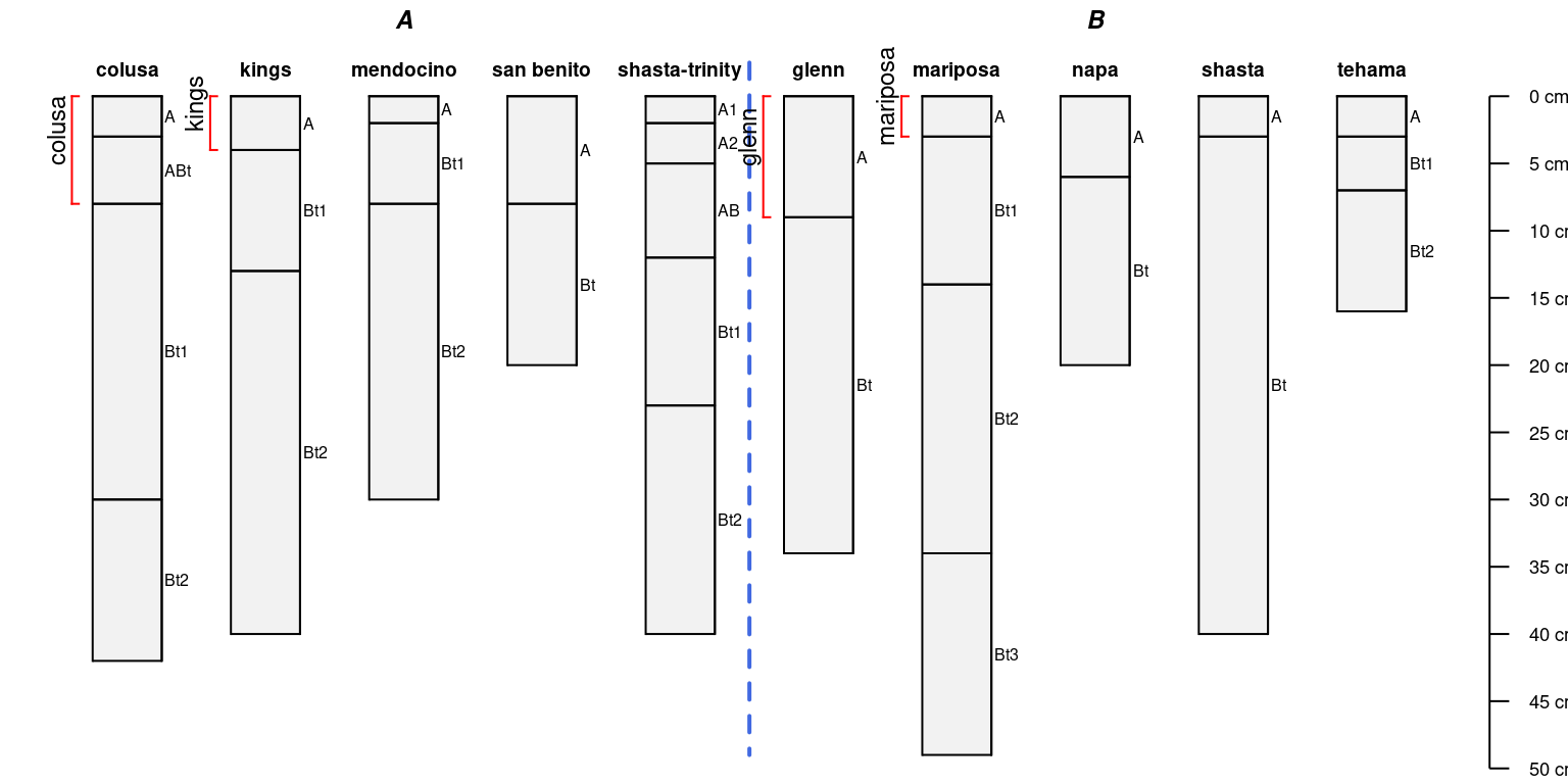

There need not be brackets for all profiles in a collection:

par(mar = c(0, 0, 0, 0))
a.sub <- a[1:4,]
groupedProfilePlot(sp4, groups = 'group')
addBracket(a.sub, col = 'red', offset = -0.4)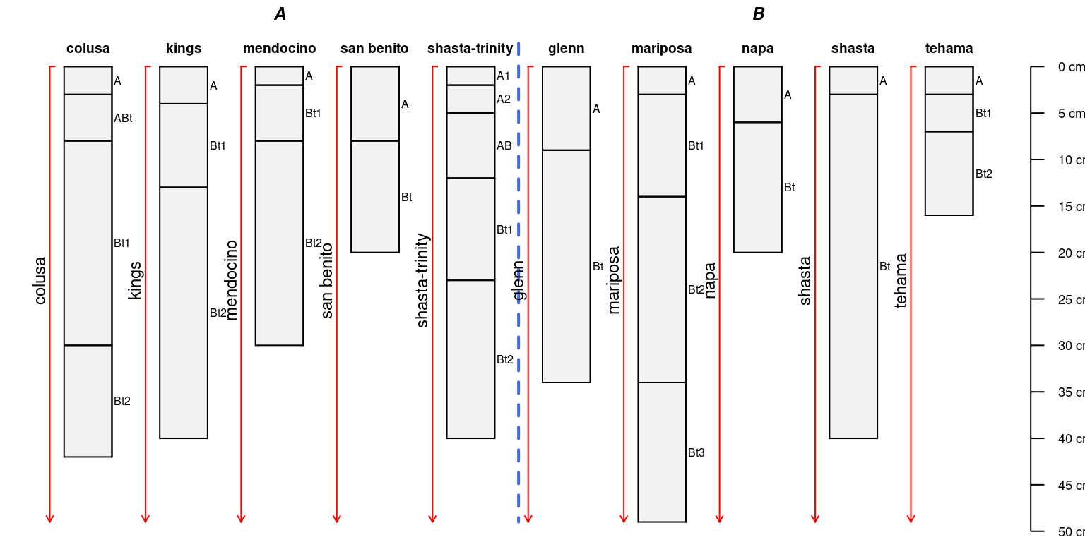

When bottom depths are missing an arrow is used:

a$bottom <- NA
par(mar = c(0, 0, 0, 0))
groupedProfilePlot(sp4, groups = 'group')
addBracket(a, col = 'red', offset = -0.4)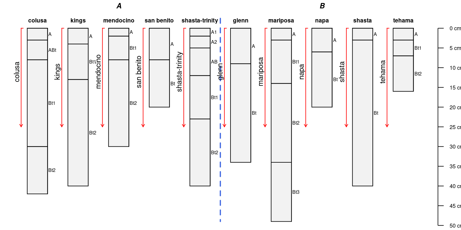

Manually define bottom depth:

par(mar = c(0, 0, 0, 0))
groupedProfilePlot(sp4, groups = 'group')
addBracket(
  a,
  col = 'red',
  label.cex = 0.75,
  missing.bottom.depth = 25,
  offset = -0.4
)

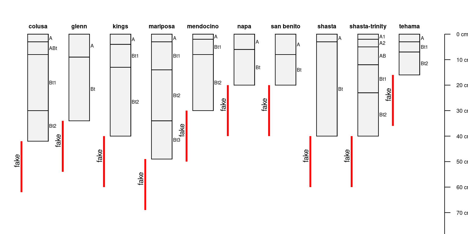
Further customization of brackets:

par(mar = c(0, 0, 0, 0))
plotSPC(sp4, max.depth = 75)

# copy root-restricting features
a <- restrictions(sp4)

# add a label: restrictive feature 'kind'
a$label <- a$kind

# add restrictions using vertical bars
addBracket(
  a,
  col = 'red',
  label.cex = 0.75,
  tick.length = 0,
  lwd = 3,
  offset = -0.4
)

Notes

These functions (addBracket(), addDiagnosticBracket(), and addVolumeFraction()) will automatically compensate for alternative sketch ordering or relative positioning of profiles.

SVG Output for Use in Page Layout Tools

Sketches for use in layout tools such as Adobe Illustrator or Inkscape should be stored in a vector file format. SVG is compatible with most software titles. WMF output is compatible with MS Office tools and can be written with the win.metafile() function.

# library(svglite)
# svglite(filename = 'e:/temp/fig.svg', width = 7, height = 6, pointsize = 12)
# 
# par(mar = c(0,2,0,4), xpd = NA)
# plotSPC(x, cex.names=1, depth.axis = list(line = -0.2), width=0.3)
# 
# dev.off()

Iterating Over Profiles in a Collection

The profileApply() function is an extension of the familiar apply() family of functions extended to SoilProfileCollection objects.

The function named in the FUN argument is evaluated once for each profile in the collection, typically returning a single value per profile. In this case, the ordering of the results would match the ordering of values in the site level attribute table.

# max() returns the depth of a soil profile
sp4$soil.depth <- profileApply(sp4, FUN = max)

# max() with additional argument give max depth to non-missing 'clay'
sp4$soil.depth.clay <- profileApply(sp4, FUN = max, v = 'clay')

# nrow() returns the number of horizons
sp4$n.hz <- profileApply(sp4, FUN = nrow)

# compute the mean clay content by profile using an inline function
sp4$mean.clay <- profileApply(sp4, FUN = function(i) mean(i$clay))

# estimate soil depth based on horizon designation
sp4$soil.depth <- profileApply(sp4, estimateSoilDepth, name = 'name')

When FUN returns a vector of the same length as the number of horizons in a profile, profileApply() can be used to create new horizon-level attributes. For example, the change in clay content by horizon depth (delta.clay, below) could be calculated as:

# save as horizon-level attribute
sp4$delta.clay <- profileApply(sp4, FUN = function(i) c(NA, diff(i$clay)))

# check results:
horizons(sp4)[1:6, c('id', 'top', 'bottom', 'clay', 'delta.clay')]

#>       id top bottom clay delta.clay
#> 1 colusa   0      3   21         NA
#> 2 colusa   3      8   27          6
#> 3 colusa   8     30   32          5
#> 4 colusa  30     42   55         23
#> 5  glenn   0      9   25         NA
#> 6  glenn   9     34   34          9

More complex summaries can be generated by writing a custom function that is then called by profileApply(). Note that each profile is passed into this function and accessed via a temporary variable (i), which is a SoilProfileCollection object containing a single profile. See help(profileApply) for details.

A list of SoilProfileCollection objects returned from a custom function can be combined into a single SoilProfileCollection object via combine().

# compute hz-thickness weighted mean exchangeable-Ca:Mg
wt.mean.ca.mg <- function(i) {
  # use horizon thickness as a weight
  thick <- i$bottom - i$top
  
  # compute the thickness weighted mean, ignoring missing values
  weighted.mean(i$ex_Ca_to_Mg, w = thick, na.rm = TRUE)
}

# apply our custom function and save results as a site-level attribute
sp4$wt.mean.ca.to.mg <- profileApply(sp4, wt.mean.ca.mg)

We can now use our some of our new site-level attributes to order the profiles when plotting.

In this case profiles are ordered based on the horizon-thickness weighted mean, exchangeable Ca:Mg values. Horizons are colored by exchangeable Ca:Mg values.

# plot the data using our new order based on Ca:Mg weighted average
# the result is an index of rank 
new.order <- order(sp4$wt.mean.ca.to.mg)

par(mar = c(4, 0, 3, 0)) # tighten figure margins
plotSPC(sp4,
        name = 'name',
        color = 'ex_Ca_to_Mg',
        plot.order = new.order)

# add an axis labeled with the sorting criteria
axis(1, at = 1:length(sp4), labels = round(sp4$wt.mean.ca.to.mg, 3), cex.axis = 0.75)
mtext(1, line = 2.25, text = 'Horizon Thickness Weighted Mean Ex. Ca:Mg', cex = 0.75)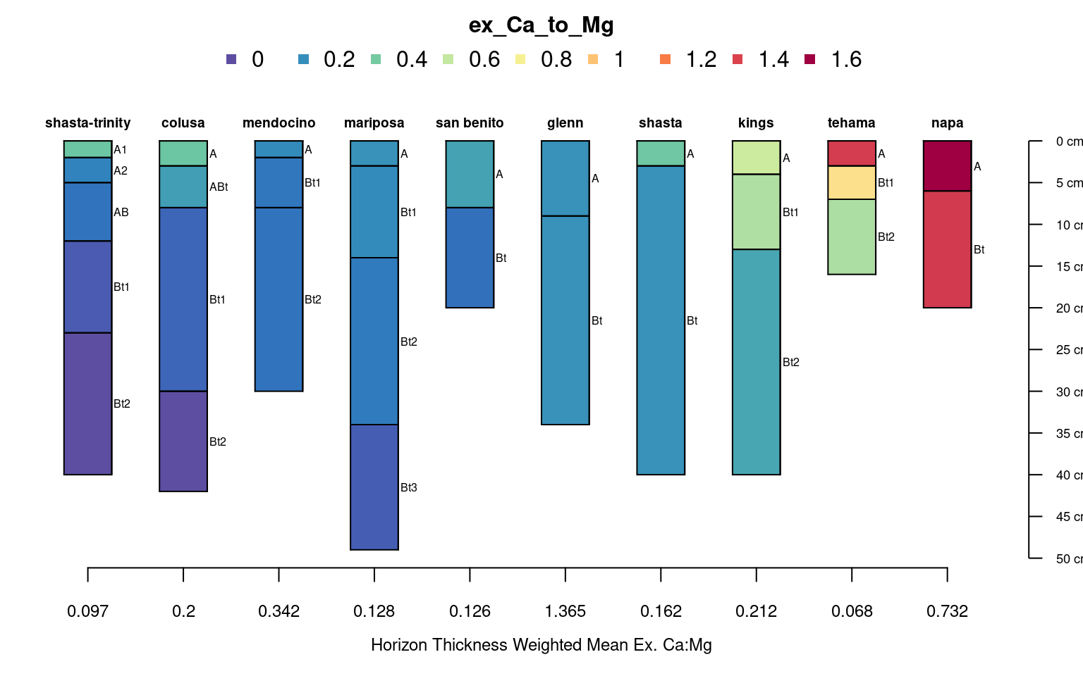

Depth-wise Selection and Resampling

Slicing Horizons: dice()

Collections of soil profiles can be sliced (or re-sampled) into regular depth-intervals with the dice() function. The slicing structure and variables of interest are defined via formula notation:

# slice select horizon-level attributes
seq ~ var.1 + var.2 + var.3 + ...
# slice all horizon-level attributes
seq ~ .

where seq is a sequence of integers (e.g. 0:15, c(5,10,15,20), etc.) and var.1 + var.2 + var.3 + ... are horizon-level attributes to slice. Both continuous and categorical variables can be named on the right-hand-side of the formula. The results returned by dice() is either a SoilProfileCollection, or data.frame when called with the optional argument SPC = FALSE. For example, to slice our sample data set into 1-cm intervals, from 0–15 cm:

# resample to 1cm slices
s <- dice(sp4, fm = 0:15 ~ sand + silt + clay + name + ex_Ca_to_Mg)

# check the result
class(s)

#> [1] "SoilProfileCollection"
#> attr(,"package")
#> [1] "aqp"

# plot sliced data
par(mar = c(0, 0, 3, 0)) # tighten figure margins
plotSPC(s, color = 'ex_Ca_to_Mg')

Once soil profile data have been sliced, it is simple to extract “chunks” of data by depth interval via [-subsetting:

# slice from 0 to max depth in the collection
s <- dice(sp4, fm= 0:max(sp4) ~ sand + silt + clay + name + ex_Ca_to_Mg)

# extract all data over the range of 5--10 cm:
plotSPC(s[, 5:10])

# extract all data over the range of 25--50 cm:
plotSPC(s[, 25:50])

# extract all data over the range of 10--20 and 40--50 cm:
plotSPC(s[, c(10:20, 40:50)])

Ragged Extraction: glom()

Select all horizons that overlap the interval of 5-15cm:

# truncate to the interval 5-15cm
clods <- glom(sp4, z1 = 5, z2 = 15)

# plot outlines of original profiles
par(mar = c(0, 0, 3, 1.5)) 
plotSPC(sp4, color = NA, name = NA, print.id = FALSE, depth.axis = FALSE, lwd = 0.5)

# overlay glom() depth criteria
rect(xleft = 0.5, ybottom = 15, xright = length(sp4) + 0.5, ytop = 5, lty = 2)

# add SoilProfileCollection with selected horizons
plotSPC(clods, add = TRUE, cex.names = 0.6, name = 'name', color = 'ex_Ca_to_Mg', name.style = 'center-center')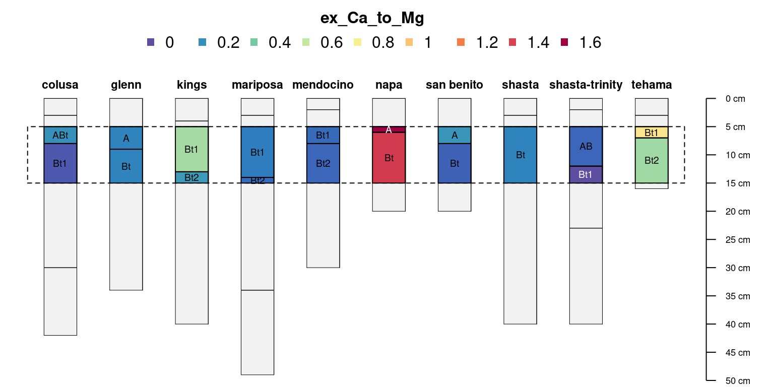

Truncation: trunc()

Truncate the SPC to the interval of 5-15cm:

# truncate to the interval 5-15cm
sp4.truncated <- trunc(sp4, 5, 15)

# plot outlines of original profiles
par(mar = c(0, 0, 3, 1.5)) 
plotSPC(sp4, color = NA, name = NA, print.id = FALSE, lwd = 0.5)

# overlay truncation criteria
rect(xleft = 0.5, ybottom = 15, xright = length(sp4) + 0.5, ytop = 5, lty = 2)

# add truncated SoilProfileCollection
plotSPC(sp4.truncated, depth.axis = FALSE, add = TRUE, cex.names = 0.6, name = 'name', color = 'ex_Ca_to_Mg', name.style = 'center-center')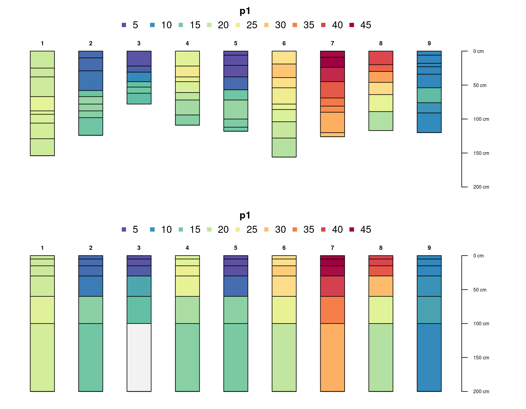

Change of Support

There is often a need for converting data to a new set of depth intervals. This re-alignment of horizon depths via aggregation can be considered a type of change of support. The operation on SoilProfileCollection objects requires some aggregation function (mean, median, etc.) and possibly interpolation (e.g. splines).

Aggregation over “slabs”

The slab() function is the simplest way to implement a change of depth support via aggregation. Profile grouping criteria and horizon attribute selection is parameterized via formula: either groups ~ var1 + var2 + var3 where named variables are aggregated within groups OR where named variables are aggregated across the entire collection ~ var1 + var2 + var3. The default summary function (slab.fun) computes the 5th, 25th, 50th, 75th, and 95th percentiles via Harrell-Davis quantile estimator.

The depth structure (“slabs”) over which summaries are computed is defined with the slab.structure argument using:

• a single integer (e.g. 10): data are aggregated over a regular sequence of 10-unit thickness slabs
• a vector of 2 integers (e.g. c(50, 60)): data are aggregated over depths spanning 50–60 units
• a vector of 3 or more integers (e.g. c(0, 5, 10, 50, 100)): data are aggregated over the depths spanning 0–5, 5–10, 10–50, 50–100 units

# aggregate a couple of the horizon-level attributes, 
# across the entire collection, 
# from 0--10 cm
# computing the mean value ignoring missing data
slab(
  sp4,
  fm = ~ sand + silt + clay,
  slab.structure = c(0, 10),
  slab.fun = mean,
  na.rm = TRUE
)

#>   variable all.profiles value contributing_fraction top bottom
#> 1     sand            1 47.63                     1   0     10
#> 2     silt            1 31.15                     1   0     10
#> 3     clay            1 21.11                     1   0     10

# again, this time within groups defined by a site-level attribute:
slab(
  sp4,
  fm = group ~ sand + silt + clay,
  slab.structure = c(0,  10),
  slab.fun = mean,
  na.rm = TRUE
)

#>   variable group value contributing_fraction top bottom
#> 1     sand     A 48.26                     1   0     10
#> 2     sand     B 47.00                     1   0     10
#> 3     silt     A 31.52                     1   0     10
#> 4     silt     B 30.78                     1   0     10
#> 5     clay     A 20.30                     1   0     10
#> 6     clay     B 21.92                     1   0     10

# again, this time over several depth ranges
slab(
  sp4,
  fm = ~ sand + silt + clay,
  slab.structure = c(0, 10, 25, 40),
  slab.fun = mean,
  na.rm = TRUE
)

#>   variable all.profiles    value contributing_fraction top bottom
#> 1     sand            1 47.63000             1.0000000   0     10
#> 2     sand            1 42.38931             0.8733333  10     25
#> 3     sand            1 32.14607             0.5933333  25     40
#> 4     silt            1 31.15000             1.0000000   0     10
#> 5     silt            1 29.41221             0.8733333  10     25
#> 6     silt            1 31.34831             0.5933333  25     40
#> 7     clay            1 21.11000             1.0000000   0     10
#> 8     clay            1 28.10687             0.8733333  10     25
#> 9     clay            1 36.26966             0.5933333  25     40

# again, this time along 1-cm slices, computing quantiles
agg <- slab(sp4, fm = ~ Mg + Ca + ex_Ca_to_Mg + CEC_7 + clay)

# see ?slab for details on the default aggregate function
head(agg)

#>   variable all.profiles  p.q5  p.q25 p.q50  p.q75 p.q95 contributing_fraction top bottom
#> 1       Mg            1 6.015 12.175 14.60 21.125 27.13                     1   0      1
#> 2       Mg            1 6.015 12.175 14.60 21.125 27.13                     1   1      2
#> 3       Mg            1 6.015 12.175 19.15 25.650 27.76                     1   2      3
#> 4       Mg            1 6.195 13.175 21.05 25.050 30.73                     1   3      4
#> 5       Mg            1 6.195 13.175 21.05 25.050 30.73                     1   4      5
#> 6       Mg            1 6.195 13.175 21.05 26.250 31.72                     1   5      6

# plot median +/i bounds defined by the 25th and 75th percentiles
# this is lattice graphics, syntax is a little rough
xyplot(top ~ p.q50 | variable, data = agg, ylab = 'Depth', 
       xlab = 'median bounded by 25th and 75th percentiles',
       lower = agg$p.q25, upper = agg$p.q75, ylim = c(42, -2),
       panel = panel.depth_function,
       alpha = 0.25, sync.colors = TRUE,
       par.settings = list(superpose.line = list(col = 'RoyalBlue', lwd = 2)), 
       prepanel = prepanel.depth_function,
       cf = agg$contributing_fraction, cf.col = 'black', cf.interval = 5,
       layout = c(5, 1), strip = strip.custom(bg = grey(0.8)),
       scales = list(x = list(
         tick.number = 4,
         alternating = 3,
         relation = 'free'
       ))
)

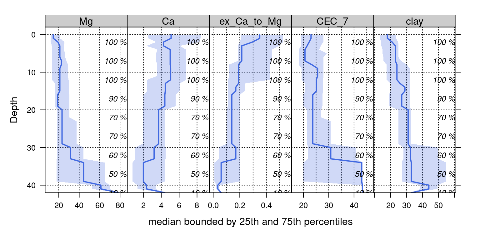
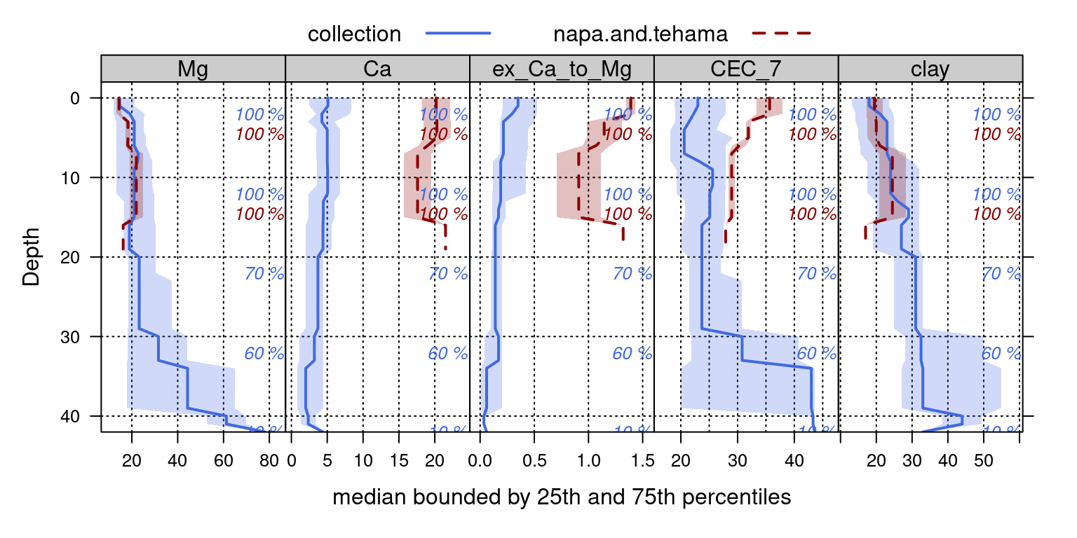
Depth-wise aggregation can be useful for visual evaluation of multivariate similarity among groups of profiles.

# processing the "napa" and tehama profiles
idx <- which(profile_id(sp4) %in% c('napa', 'tehama'))
napa.and.tehama <- slab(sp4[idx,], fm = ~ Mg + Ca + ex_Ca_to_Mg + CEC_7 + clay)

# combine with the collection-wide aggregate data
g <- make.groups(collection = agg, napa.and.tehama = napa.and.tehama)

# compare graphically:
xyplot(top ~ p.q50 | variable, groups = which, data = g, ylab = 'Depth',
       xlab = 'median bounded by 25th and 75th percentiles',
       lower = g$p.q25, upper = g$p.q75, ylim = c(42, -2),
       panel = panel.depth_function,
       alpha = 0.25, sync.colors = TRUE, cf = g$contributing_fraction, cf.interval = 10,
       par.settings = list(superpose.line = list(
         col = c('RoyalBlue', 'Red4'),
         lwd = 2,
         lty = c(1, 2)
       )),
       prepanel = prepanel.depth_function,
       layout = c(5, 1), 
       strip = strip.custom(bg = grey(0.8)),
       scales = list(x = list(
         tick.number = 4,
         alternating = 3,
         relation = 'free'
       )),
       auto.key = list(columns = 2,
                       lines = TRUE,
                       points = FALSE)
)

The following example is based on a set of 9 randomly generated profiles, re-aligned to the Global Soil Map (GSM) standard depths.

library(data.table)
library(RColorBrewer)

# 9 random profiles
# 1 simulated property via logistic power peak (LPP) function
# 6, 7, or 8 horizons per profile
# result is a list of single-profile SPC
d <- lapply(
  as.character(1:9), 
  random_profile, 
  n = c(6, 7, 8), 
  n_prop = 1, 
  method = 'LPP',
  SPC = TRUE
)

# combine into single SPC
d <- combine(d)

# GSM depths
gsm.depths <- c(0, 5, 15, 30, 60, 100, 200)

# aggregate using mean: wt.mean within slabs
# see ?slab for ideas on how to parameterize slab.fun
d.gsm <- slab(d, fm = id ~ p1, slab.structure = gsm.depths, slab.fun = mean, na.rm = TRUE)

# note: result is in long-format
# note: horizon names are lost due to aggregation
head(d.gsm, 7)

#>   variable id    value contributing_fraction top bottom
#> 1       p1  1 45.44919             1.0000000   0      5
#> 2       p1  1 52.60948             1.0000000   5     15
#> 3       p1  1 50.62579             1.0000000  15     30
#> 4       p1  1 46.70293             1.0000000  30     60
#> 5       p1  1 37.54221             1.0000000  60    100
#> 6       p1  1 31.23363             0.7826087 100    200
#> 7       p1  2 16.26688             1.0000000   0      5

A simple graphical comparison of the original and re-aligned soil profile data, after converting slab() result from long -> wide format with {data.table} dcast():

# reshape to wide format
# this scales to > 1 aggregated variables
d.gsm.pedons <- data.table::dcast(
  data.table(d.gsm), 
  formula = id + top + bottom ~ variable, 
  value.var = 'value'
  )

# init SPC
depths(d.gsm.pedons) <- id ~ top + bottom

# iterate over aggregated profiles and make new hz names
d.gsm.pedons$hzname <- profileApply(d.gsm.pedons, function(i) {
  paste0('GSM-', 1:nrow(i))
})

# compare original and aggregated
par(mar = c(1, 0, 3, 3), mfrow = c(2, 1))
plotSPC(d, color = 'p1')
mtext('original depths', side = 2, line = -1.5)
plotSPC(d.gsm.pedons, color = 'p1')
mtext('GSM depths', side = 2, line = -1.5)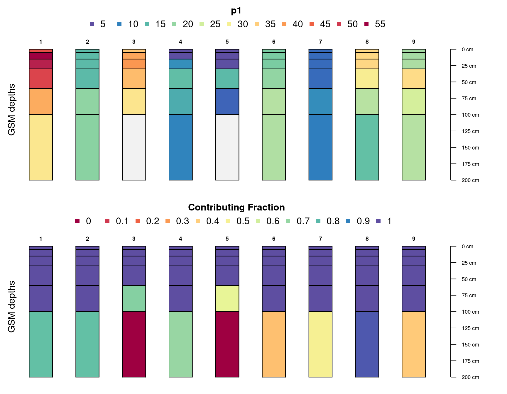

Note that re-aligned data may not represent reality (and should therefore be used with caution) when the original soil depth is shallower than the deepest of the new (re-aligned) horizon depths. The contributing_fraction metric returned by slab() can be useful for assessing how much real data were used to generate the new set of re-aligned data.

# reshape to wide format
d.gsm.pedons.2 <- data.table::dcast(
  data.table(d.gsm), 
  formula = id + top + bottom ~ variable, 
  value.var = 'contributing_fraction'
)

# init SPC
depths(d.gsm.pedons.2) <- id ~ top + bottom

# compare original and aggregated
par(mar = c(1, 0, 3, 3), mfrow = c(2, 1))
plotSPC(d.gsm.pedons, name = '', color = 'p1')
mtext('GSM depths', side = 2, line = -1.5)

plotSPC(
  d.gsm.pedons.2,
  name = '',
  color = 'p1',
  col.label = 'Contributing Fraction',
  col.palette = RColorBrewer::brewer.pal(10, 'Spectral')
)
mtext('GSM depths', side = 2, line = -1.5)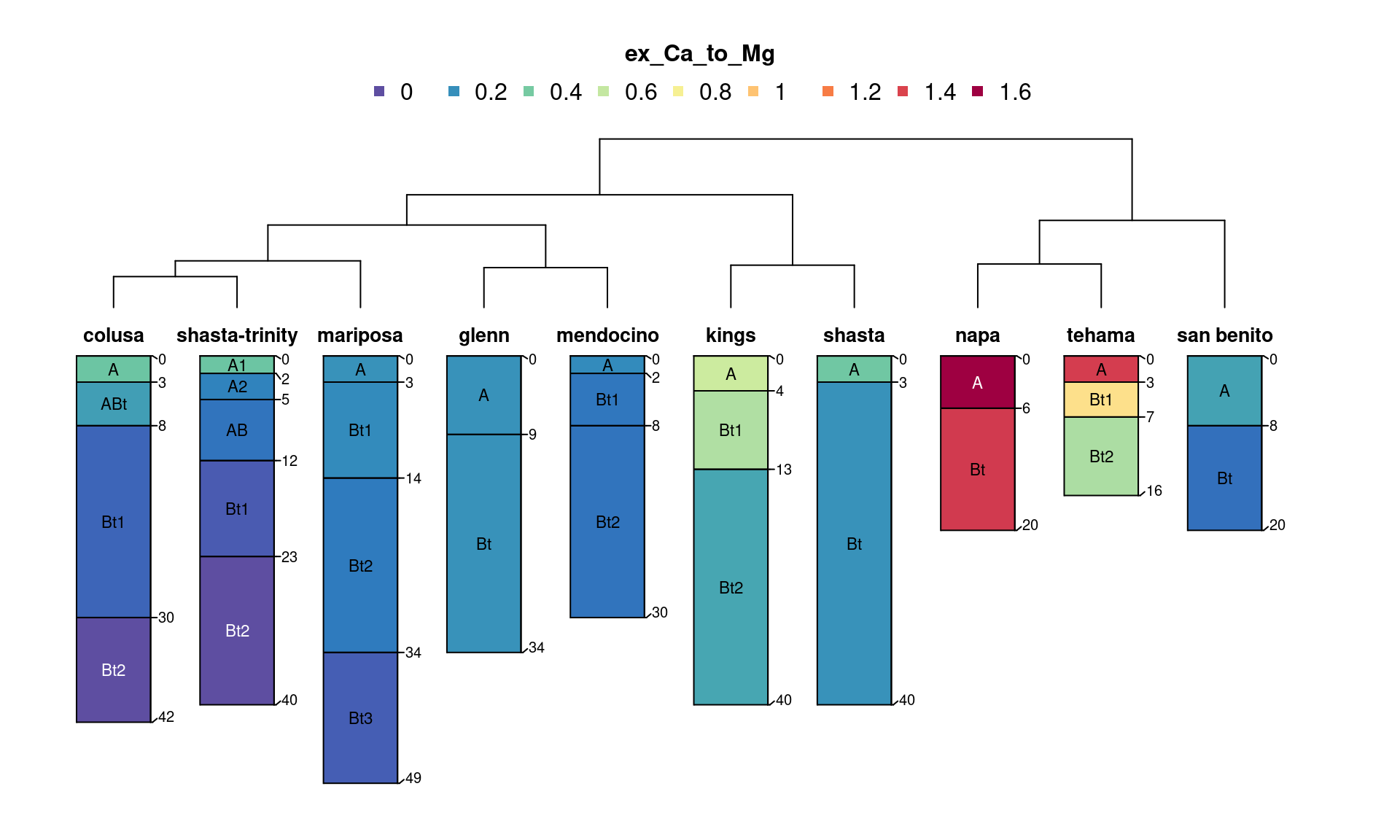

Pair-Wise Dissimilarity: NCSP()

Calculation of between-profile dissimilarity is performed using NCSP() (Numerical Classification of Soil Profiles). As of aqp 2.0, NCSP() replaces the older implementation in profile_compare() which is now deprecated. Dissimilarity values depend on attributes selection (e.g. clay, CEC, pH , etc.), optional depth-weighting parameter (k), and a maximum depth of evaluation (maxDepth).

See the function manual page and this paper for details.

library(cluster)
library(sharpshootR)

# start fresh
data(sp4)
depths(sp4) <- id ~ top + bottom
hzdesgnname(sp4) <- 'name'

# eval dissimilarity:
# using Ex-Ca:Mg ratio and CEC at pH 7
# no depth-weighting (k = 0)
# to a maximum depth of 40 cm
d <- NCSP(sp4, vars = c('ex_Ca_to_Mg', 'CEC_7'), k = 0, maxDepth = 40)

# check distance matrix:
round(d, 1)

#>                colusa glenn kings mariposa mendocino napa san benito shasta shasta-trinity
#> glenn            13.8                                                                     
#> kings            16.0  13.1                                                               
#> mariposa          8.4  11.6  16.5                                                         
#> mendocino        12.1   8.2  17.0     15.5                                                
#> napa             31.5  24.9  30.5     30.3      22.2                                      
#> san benito       26.8  21.4  27.4     29.3      16.4 18.0                                 
#> shasta           17.2  13.6   8.7     17.6      17.6 34.8       23.3                      
#> shasta-trinity    6.4  16.9  22.3      9.6      17.0 30.9       28.3   23.3               
#> tehama           30.1  23.9  29.2     28.6      20.8  9.0       15.3   32.7           29.2

# visualize dissimilarity matrix via divisive hierarchical clustering
d.diana <- diana(d)

# this function is from the sharpshootR package
# requires some manual adjustments
par(mar = c(0, 0, 4, 0))
plotProfileDendrogram(
  sp4,
  d.diana,
  scaling.factor = 0.9,
  y.offset = 5,
  cex.names = 0.7,
  width = 0.3,
  color = 'ex_Ca_to_Mg',
  name.style = 'center-center',
  hz.depths = TRUE,
  depth.axis = FALSE
)

Some additional examples can be found in:

• Pair-Wise Distances by Generalized Horizon Labels
• Competing Soil Series
• Soil Profile Distances

---

This document is based on aqp version 2.1.0.