Chapter 4 Linear Regression
4.1 Introduction
Linear regression models the linear relationship between a response variable (y) and an predictor variable (x).
\(y = \alpha + \beta x + e\)
Where:
\(y\) = the dependent variable
\(\alpha\) = the intercept of the fitted line
\(\beta\) = the Regression coefficient, i.e. slope of the fitted line. Strong relationships will have high values.
\(x\) = the independent variable (aka explanatory or predictor variable(s) )
\(e\) = the error term
Linear regression has been used for soil survey applications since the early 1900s when Briggs, McLane, and United States. Bureau of Soils (1907) developed a pedotransfer function to estimate the wilting coefficient as a function of soil particle size.
Wilting coefficient = 0.01(sand) + 0.12(silt) + 0.57(clay)
When more than one independent variable is used in the regression, it is referred to as multiple linear regression. In regression models, the response (or dependent) variable must always be continuous. The predictor (or independent) variable(s) can be continuous or categorical. In order to use linear regression or any linear model, the errors (i.e. residuals) must be normally distributed. Most environmental data are skewed and require transformations to the response variable (such as square root or log) for use in linear models. Normality can be assessed using a QQ plot or histogram of the residuals.
4.2 Linear Regression Example
Now that we’ve got some of the basic theory out of the way we’ll move on to a real example, and address any additional theory where it relates to specific steps in the modeling process. The example selected for this chapter comes from the Mojave desert. The landscape is composed primarily of closed basins ringed by granitic hills and mountains (Peterson, 1981). The problem tackled here is modeling mean annual air temperature as a function of PRISM, digital elevation model (DEM) and Landsat derivatives.
This climate study began in 1998 as part of a national study run by the National Lab and led by Henry Mount (Mount and Paetzold 2002). The objective was to determine if the hyperthermic line was consistent across the southern US, which at the time was thought to be ~3000 in elevation. Up until 2015 their were 77 active MAST sites, and 12 SCAN sites throughout MLRA 30 and 31.
For more details see the “MLRA 30 - Soil Climate Study - Soil Temperature” project in NASIS, on GitHub, or by (Roecker and Carrie-Ann Haydu-Houdeshell 2012).
## Loading required namespace: rvest## mlrassoarea nonmlrassaarea mlraarea projecttypename projectsubtypename
## 4 SW-VIC <NA> 30 MLRA <NA>
## fiscalyear fiscalyear_goaled projectiid uprojectid
## 4 2015 2015 95689 0000-VIC-Soil Climate Studies-001
## projectname projectapprovedflag
## 4 MLRA 30 - Soil Climate Study - Soil Temperature TRUE
## projectconcerntypename
## 4 <NA>
## projectdesc
## 4 8-VIC, Victorville, CA MLRA Soil Survey Office\r\nSoil Climate Study Plan \r\nProject Outline Worksheet \r\n\r\nProject Name: MLRA 30 and 31 - Soil Climate Study Plan\r\n\r\nIdentification \r\nState/s: CA and NV (proposed to add in AZ as well)\r\nMLRAs: 30 and 31\r\nPlan Author: Carrie-Ann Houdeshell, MLRA SSPL and Stephen Roecker Soil Scientist\r\nRegional Office Staff: \r\nDavis, CA: Ed Tallyn, Senior Regional Soil Scientist; Jennifer Wood, Soil Data Quality Specialist\r\nPhoenix, AZ: Nathan Starman, Soil Data Quality Specialist\r\nArea Office Staff: Peter Fahnestock, Area Resource Soil Scientist\r\n\r\nProject Contact Person(s) \r\nName: Carrie-Ann Houdeshell or Stephen Roecker\r\naddress: 15415 W. Sand St. #103, Victorville, CA 92392\r\nphone: (760) 843-6882\r\nemail: Carrie-Ann.Houdeshell@ca.usda.gov or Stephen.Roecker@ca.usda.gov\r\n\r\nProject Objective(s) \r\nThe original objective of this study was to determine the thermic/hyperthermic boundary across MLRA 30. Currently the primary objective is to estimate soil tempe...
## n_projectdesc n_areasymbol n_nationalmusym n_spatial date_start date_complete
## 4 13724 NA NA NA <NA> <NA>
## date_qc date_qa_start date_qa_complete date_qc_spatial date_qa_spatial
## 4 <NA> <NA> <NA> <NA> <NA>
## pl_username qa_username muacres acre_landcat acre_goal acre_progress
## 4 Ballmer, Matthew <NA> NA NA 0 0
## pct_progress muacres_water acre_water acre_prog_water acre_federal
## 4 NA NA NA NA NA
## acre_prog_federal acre_private acre_prog_private acre_native acre_prog_native
## 4 NA NA NA NA NAIn addition to the 11-IND MAST modeling efforts there has also been two published studies on the Mojave. The first was by Schmidlin, Peterson, and Gifford (1983) who examined both the Great Basin and Mojave Deserts in Nevada. The second was by Bai et al. (2010) who examined the Mojave Desert in California. Both studies developed regression models using elevation, but Schmidlin, Peterson, and Gifford (1983) also incorporated latitude. The results from Bai et al. (2010) displayed considerably larger areas of hyperthermic soils than Schmidlin, Peterson, and Gifford (1983). This made be due to the unconventional method used by Bai et al. (2010) to measure MAST.
4.3 Data
4.3.1 Henry Mount Database
The Henry Mount Database already has 79 of the sites from the Mojave. However only 8 have temperature records.
## computing un-biased soil temperature summaries## 79 sensors loaded (1.89 Mb transferred)4.3.2 Aggregate Time Series
For our purposes the daily soil temperature measurements need to be aggregated to the mean annual soil temperature (MAST). However, depending data you query using, fetchHenry() maybe able to return pre-aggregated results using the gran function argument.
# extract the site and sensor data frames from the list
ms_df <- f$soiltemp
s     <- f$sensors


# rename 2 columns
ms_df <- mutate(
  ms_df,
  day  = date_time,
  Jday = doy
  )


# Plot sites visually inspect for flat lines and spikes
ms_df %>%
  filter(name == "JVOHV2-50") %>%
  ggplot(aes(x = day, y = sensor_value)) +
  geom_line()
## Warning: Removed 649 rows containing missing values or values outside the scale range
## (`geom_line()`).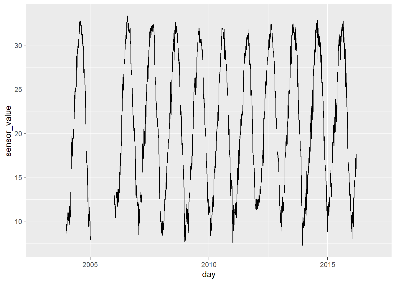
# Aggregate by Year, Month, and Julian day (i.e. 1-365, 366 for leap years)
# compute number of days per site
ms_n_df <- ms_df %>%
  group_by(sid, day) %>%
  summarise(mast = mean(sensor_value, na.exclude = TRUE)) %>%
  group_by(sid) %>%
  summarise(numDays = sum(!is.na(mast)), ) %>%
  ungroup()
## `summarise()` has regrouped the output.
## ℹ Summaries were computed grouped by sid and day.
## ℹ Output is grouped by sid.
## ℹ Use `summarise(.groups = "drop_last")` to silence this message.
## ℹ Use `summarise(.by = c(sid, day))` for per-operation grouping
## (`?dplyr::dplyr_by`) instead.# compute mast per year
ms_site_df <- ms_df %>%
group_by(sid, Jday) %>%
summarise(mast = mean(sensor_value, na.rm = TRUE)) %>%
group_by(sid) %>%
summarise(mast = mean(mast, na.rm = TRUE)) %>%
ungroup()## `summarise()` has regrouped the output.
## ℹ Summaries were computed grouped by sid and Jday.
## ℹ Output is grouped by sid.
## ℹ Use `summarise(.groups = "drop_last")` to silence this message.
## ℹ Use `summarise(.by = c(sid, Jday))` for per-operation grouping
## (`?dplyr::dplyr_by`) instead.# merge mast & numDays
mast_df <- as.data.frame(s) %>%
select(name, sid, sensor_depth, geometry) %>%
left_join(ms_site_df, by = "sid") %>%
left_join(ms_n_df, by = "sid") %>%
filter(sensor_depth == 50 & !is.na(mast))
head(mast_df)## name sid sensor_depth geometry mast numDays
## 1 JTNP15 923 50 POINT (-116.01 34.02) 19.97123 321
## 2 JAWBONE01 903 50 POINT (-117.99 35.5) 19.40847 3742
## 3 JAWBONE02 972 50 POINT (-118.14 35.5) 19.27930 3063
## 4 JVOHV1 924 50 POINT (-116.47 34.52) 21.89822 4461
## 5 JVOHV2 925 50 POINT (-116.64 34.52) 21.13497 4091
## 6 DEVA01 971 50 POINT (-116.9 36.3) 28.20590 253Note that we have a column in result data.frame called "geometry" since we created it from an sf object.
4.4 Spatial data
4.4.1 Plot Coordinates
Where do our points plot? To start we need to convert them to a spatial object first. Then we can create an interactive we map using mapview. Also, if we wish we can also export the locations as a Shapefile.
4.4.2 Extracting Spatial Data
Prior to any spatial analysis or modeling, you will need to develop a suite of geodata files that can be intersected with your field data locations. This is, in and of itself a difficult task and should be facilitated by your Regional GIS Specialist. The geodata files typically used would consist of derivatives from a DEM or satellite imagery, and a ‘good’ geology map. Prior to any prediction it is also necessary to ensure the geodata files have the same projection, extent, and cell size. Once we have the necessary files we can construct a list in R of the file names and paths, read the geodata into R, and then extract the geodata values where they intersect with field data.
As you can see below their are numerous variables we could inspect.
## Loading required package: sp## Warning: package 'sp' was built under R version 4.5.2##
## Attaching package: 'raster'## The following object is masked from 'package:dplyr':
##
## selectlibrary(sf)
# load raster stack from GitHub
githubURL <- url("https://raw.githubusercontent.com/ncss-tech/stats_for_soil_survey/master/data/mast_mojave_rs.rds")
geodata_r <- readRDS(githubURL)
# Extract the geodata and add to a data frame
mast_sf <- st_transform(mast_sf, crs = 5070)
data <- raster::extract(geodata_r, st_coordinates(mast_sf))
data <- cbind(st_drop_geometry(mast_sf), data)
# convert aspect
data$northness <- abs(180 - data$aspect)
# random sample
vars <- c("elev", "temp", "precip", "solar", "tc_1", "twi")
idx <- which(names(geodata_r) %in% vars)
geodata_s <- sampleRegular(geodata_r[[idx]], size = 1000)4.5 Exploratory Data Analysis (EDA)
Generally before we begin modeling it is good to explore the data. By examining a simple summary we can quickly see the breakdown of our data. It is important to look out for missing or improbable values. Probably the easiest way to identify peculiarities in the data is to plot it.
## siteid mast numDays elev slope
## Cheme01 : 1 Min. : 3.10 Min. : 363 Min. : 0.0 Min. : 0.00
## Clark01 : 1 1st Qu.:18.50 1st Qu.:1831 1st Qu.: 699.2 1st Qu.: 2.00
## DEVA01 : 1 Median :20.57 Median :2918 Median : 947.5 Median : 5.00
## DEVA02 : 1 Mean :19.93 Mean :2465 Mean :1082.0 Mean :11.85
## DEVA03 : 1 3rd Qu.:23.72 3rd Qu.:3397 3rd Qu.:1480.2 3rd Qu.:21.00
## Jawbone01: 1 Max. :28.77 Max. :4159 Max. :3021.0 Max. :42.00
## (Other) :62
## aspect twi solar solarcv
## Min. : 6.00 Min. : 8.00 Min. :1758 Min. :21.00
## 1st Qu.: 90.25 1st Qu.: 9.25 1st Qu.:2028 1st Qu.:31.00
## Median :140.00 Median :12.00 Median :2091 Median :32.50
## Mean :143.62 Mean :12.00 Mean :2084 Mean :32.66
## 3rd Qu.:196.00 3rd Qu.:14.00 3rd Qu.:2136 3rd Qu.:33.25
## Max. :333.00 Max. :21.00 Max. :2443 Max. :44.00
## NA's :2
## tc_1 tc_2 tc_3 precip
## Min. : 58.00 Min. : 26.00 Min. : 2.00 Min. : 3.000
## 1st Qu.: 97.75 1st Qu.: 47.75 1st Qu.: 31.50 1st Qu.: 6.000
## Median :120.00 Median : 57.50 Median : 50.50 Median : 7.000
## Mean :122.22 Mean : 56.85 Mean : 51.87 Mean : 9.824
## 3rd Qu.:143.50 3rd Qu.: 64.00 3rd Qu.: 74.00 3rd Qu.:10.000
## Max. :191.00 Max. :100.00 Max. :121.00 Max. :44.000
##
## temp northness
## Min. :10.00 Min. : 0.00
## 1st Qu.:20.75 1st Qu.: 23.75
## Median :23.50 Median : 68.00
## Mean :23.10 Mean : 64.59
## 3rd Qu.:26.00 3rd Qu.: 93.50
## Max. :31.00 Max. :174.00
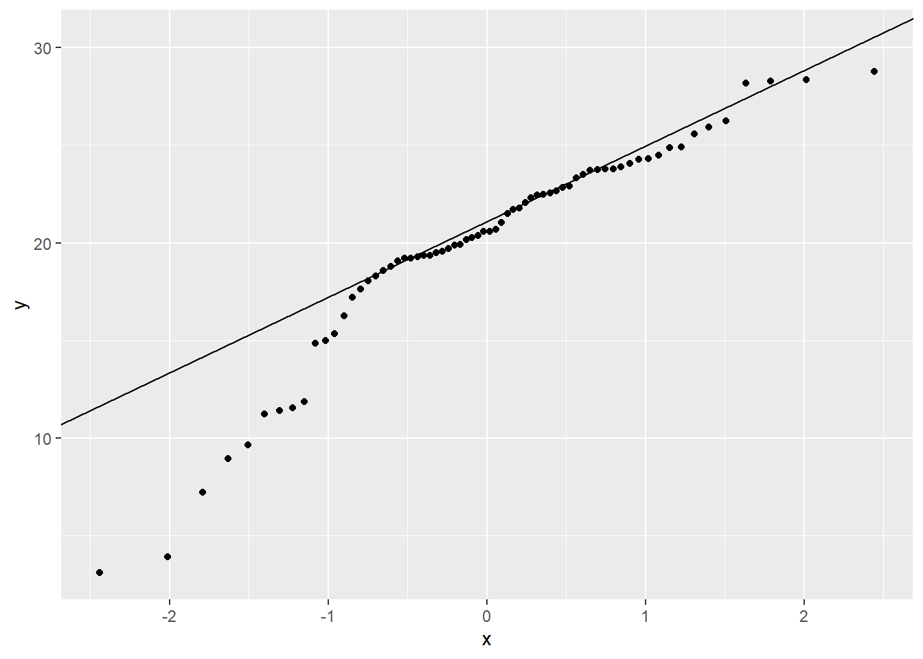
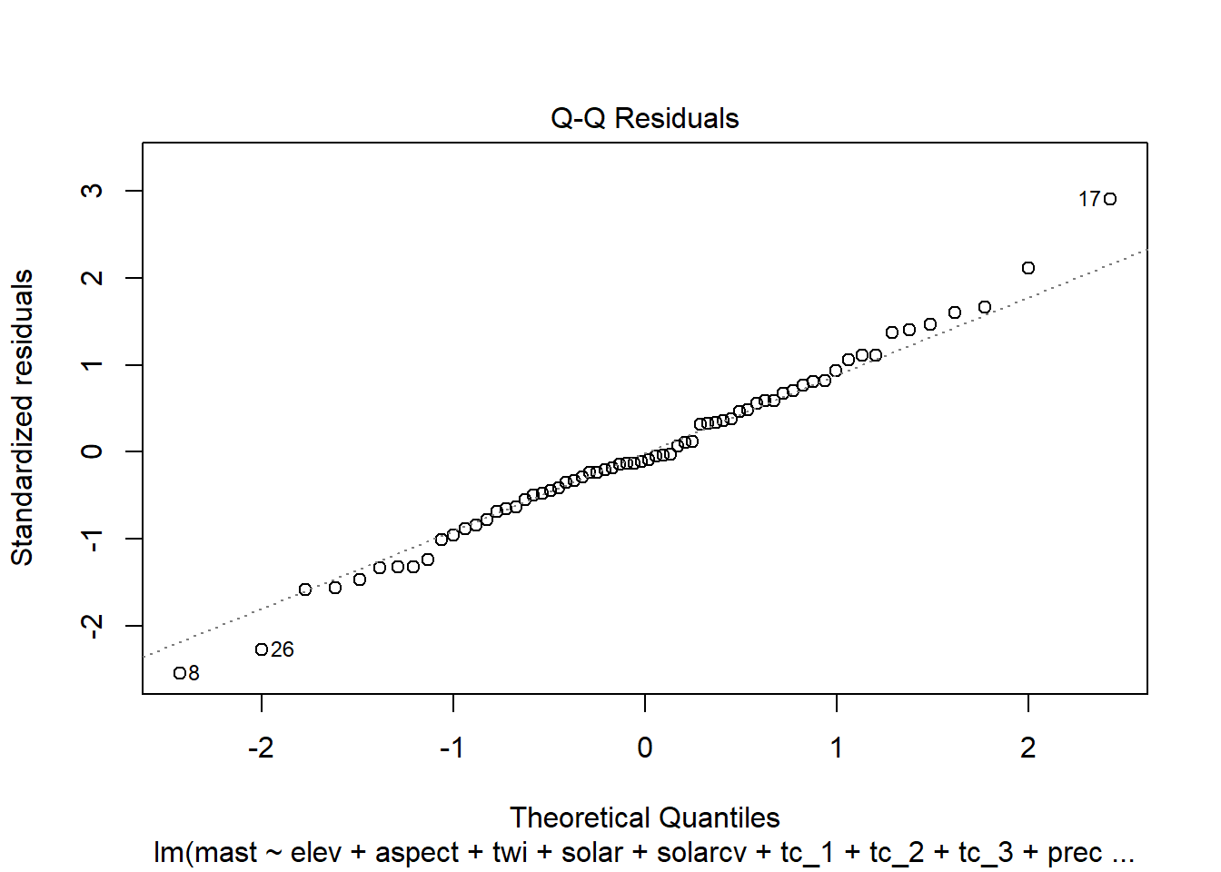
## You may recall from discussion of EDA that QQ plots are a visual way to inspect the normality of a variable. If the variable is normally distributed, the points (e.g. soil observations) should line up along the straight line.
By examining the correlations between some of the predictors we can also determine whether they are collinear (e.g. > 0.6). This is common for similar variables such as Landsat bands, terrain derivatives, and climatic variables. Variables that are colinear are redundant and contain no additional information. In addition, collinearity will make it difficult to estimate our regression coefficients.
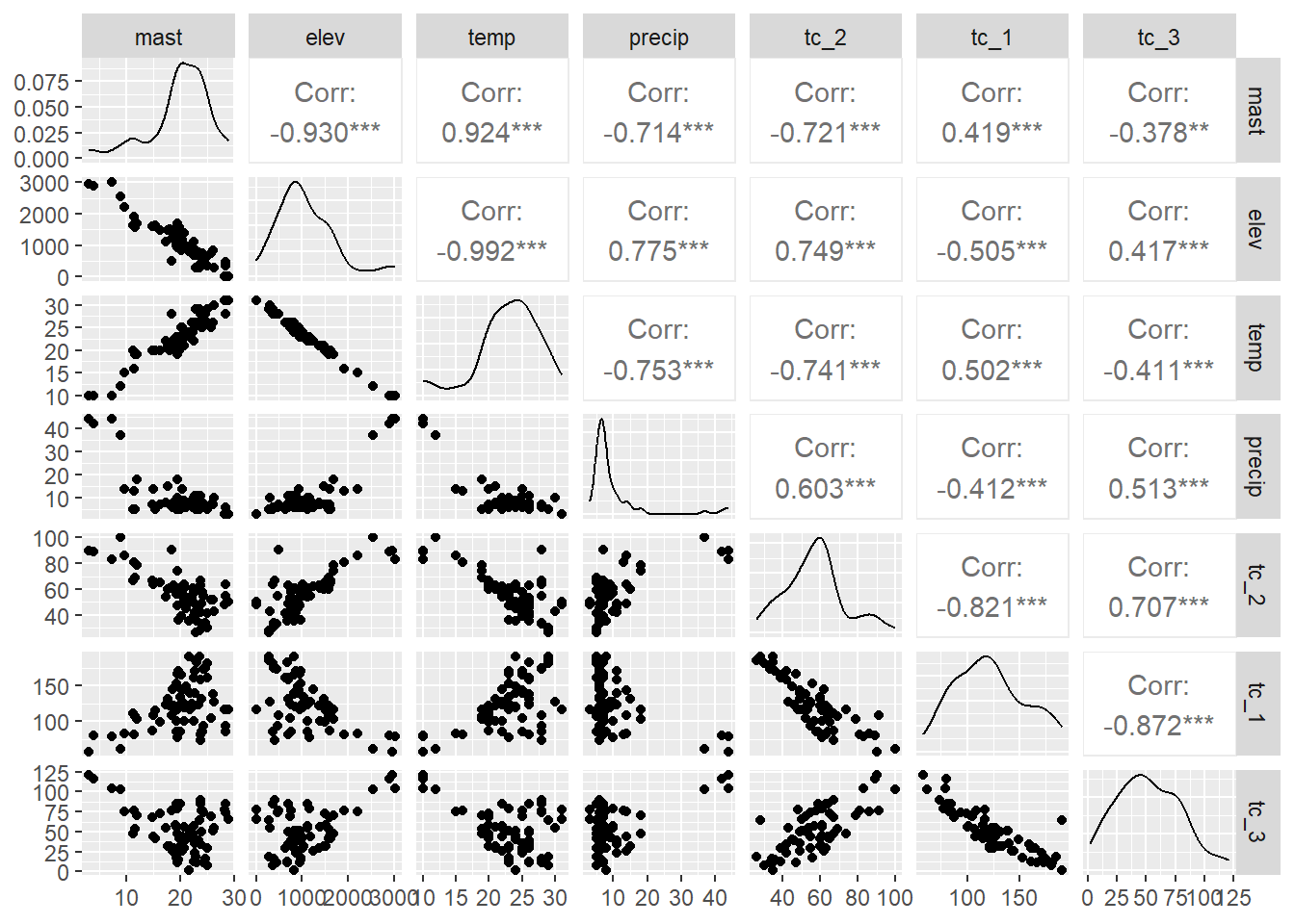
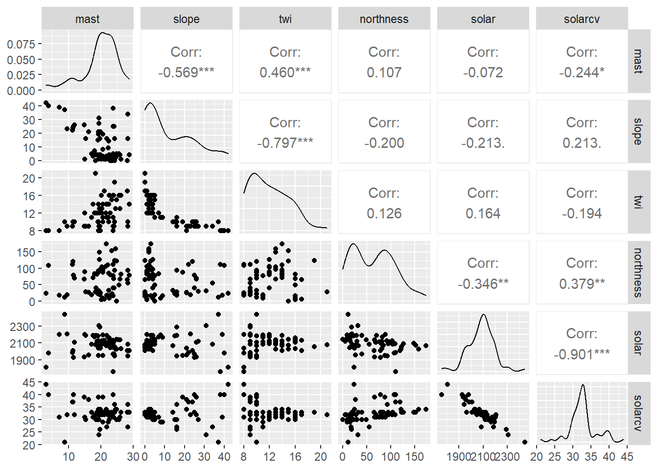
The correlation matrices and scatter plots above show that that MAST has moderate correlations with some of the variables, particularly the elevation and the climatic variables.
Examining the density plots on the diagonal axis of the scatter plots we can also see that some variables are skewed.
4.5.1 Compare Samples vs Population
Since our data was not randomly sampled, we had better check the distribution of our samples vs the population. We can accomplish this by overlaying the sample distribution of predictor variables vs a large random sample.
geodata_df <- as.data.frame(geodata_s)

geodata_df <- rbind(
  data.frame(source = "sample",     data[names(geodata_df)]),
  data.frame(source = "population", geodata_df)
)

geodata_l <- pivot_longer(geodata_df,
                          cols = -source)

ggplot(geodata_l, aes(x = value, fill = source)) +
  geom_density(alpha = 0.5) +
  facet_wrap(~ name, scales = "free") +
  ggtitle("Evaluation of Sample Representativeness")
## Warning: Removed 1266 rows containing non-finite outside the scale range
## (`stat_density()`).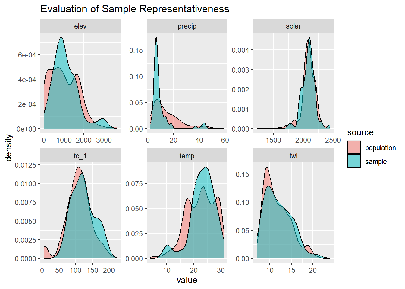
The overlap between our sample and the population appear satisfactory.
4.6 Linear modeling
R has several functions for fitting linear models. The most common is arguably the lm() function from the stats R package, which is loaded by default. The lm() function is also extended through the use of several additional packages such as the car and caret R packages. Another noteworthy R package for linear modeling is rms, which offers the ols() function for linear modeling. The rms R package (Harrell 2015) offers an ‘almost’ comprehensive alternative to `lm()’ and it’s accessory function. Each function offers useful features, therefore for the we will demonstrate elements of both. Look for comments (i.e. #) below referring to rms or stats.
# stats
fit_lm <- lm(
  formula = mast ~ elev + aspect + twi + solar + solarcv + tc_1 + tc_2 + tc_3 + precip + temp,
  data = data,
  weights = data$numDays
  )


# rms R package

library(rms)

dd <- datadist(data)
options(datadist = "dd")

fit_ols <- ols(mast ~ elev + aspect + twi + solar + solarcv + tc_1 + tc_2 + tc_3 + precip + temp, data = data, x = TRUE, y = TRUE, weights = data$numDays)
4.6.1 Diagnostics
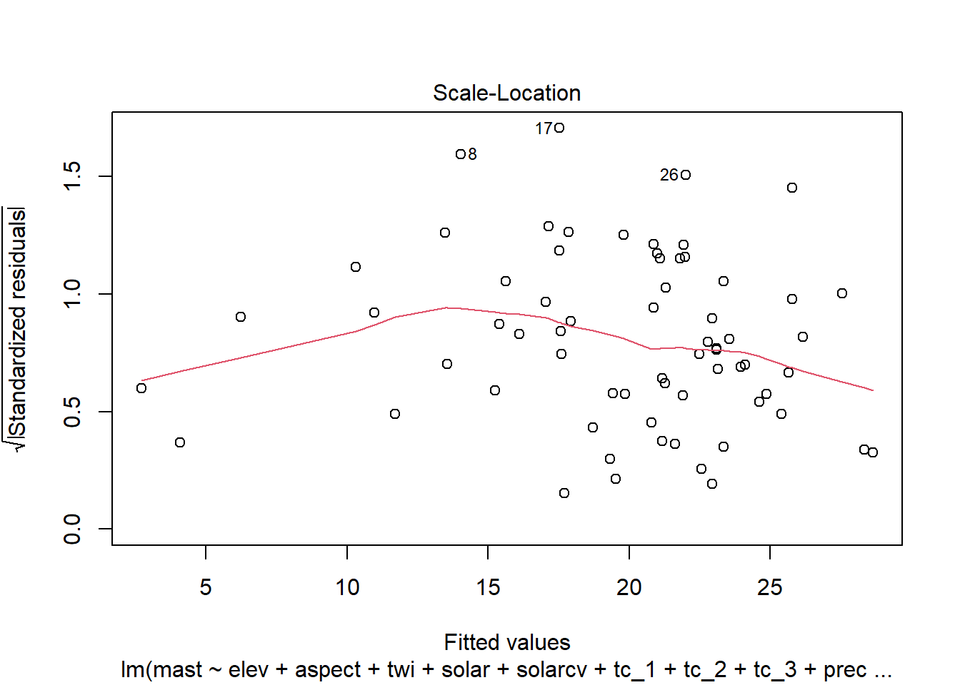
4.6.1.1 Residual plots
Once we have a model we need to assess residuals for linearity, normality, and homoscedastivity (or constant variance). Oddly this is one area were the rms R package does not offer convenient functions for plotting residuals, therefore we’ll simply access the results of lm().
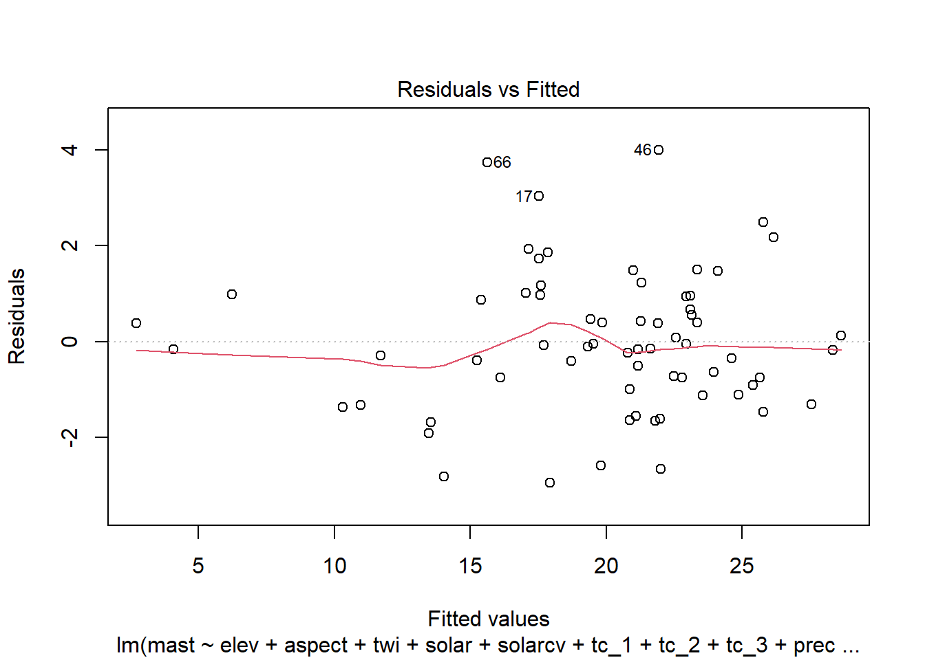
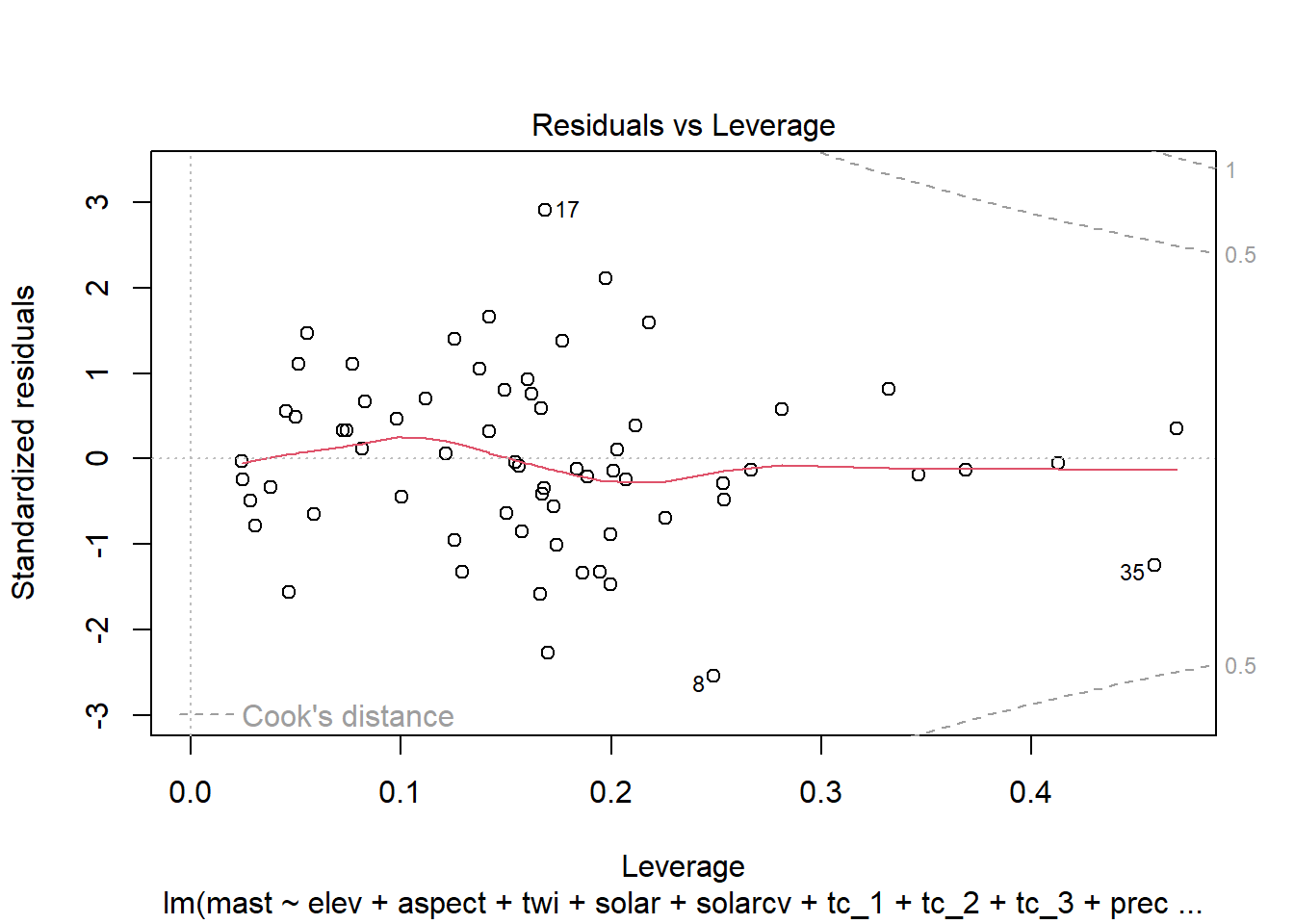
Remember the residuals are simply just the observed values minus the predicted values, which are easy enough to calculate. Alternatively we can simply extract them from the fitted model object.
##          1          2          3          4          5          6
## -1.3182498 -0.4111067 0.1231537 1.4750626 -0.1719747 -0.1036808## 1 2 3 4 5 6
## -1.3182498 -0.4111067 0.1231537 1.4750626 -0.1719747 -0.10368084.6.1.2 Multicolinearity
As we mentioned earlier multicolinearity should be avoided. To assess a model for multicolinearity we can compute the variance inflation factor (VIF). Its square root indicates the amount of increase in the predictor coefficients standard error. A value greater than 3 indicates a doubling the standard error. Rules of thumb vary, but a square root of vif greater than 2 or 3 indicates an unacceptable value (Faraway 2004).
##     elev   aspect      twi    solar  solarcv     tc_1     tc_2     tc_3
## 8.851106 1.103580 2.056235 6.068831 5.787921 4.114079 3.009392 3.311669
##   precip     temp
## 2.274489 7.860236## elev aspect twi solar solarcv tc_1 tc_2 tc_3 precip temp
## TRUE FALSE FALSE TRUE TRUE TRUE TRUE TRUE FALSE TRUEThe values above indicate we have several colinear variables in the model, which you might have noticed already from the scatter plot matrix.
4.6.2 Variable selection/reduction
Modeling is an iterative process that cycles between fitting and evaluating alternative models. Compared to tree and forest models, linear and generalized models are typically less automated. Automated model selection procedures are available, but should not be taken at face value because they may result in complex and unstable models. This is in part due to correlation amongst the predictive variables that can confuse the model. Also, the order in which the variables are included or excluded from the model effects the significance of the other variables, and thus several weak predictors might mask the effect of one strong predictor. Regardless of the approach used, variable selection is probably the most controversial aspect of linear modeling.
- Step-wise selection (
step(),rms::validate()) - Principal component analysis (
princomp()) - Shrinkage methods (e.g. Lasso)
- Randomized wrapper (e.g. Boruta)(
Boruta::Boruta())
Both the rms and caret packages offer methods for variable selection and cross-validation. In this instance the rms approach is a bit more convenient, with the one line call to validate().
# Set seed for reproducibility
set.seed(42)


# rms
## stepwise selection
validate(fit_ols, bw = TRUE)
##
## Backwards Step-down - Original Model
##
## Deleted Chi-Sq d.f. P Residual d.f. P AIC R2
## temp 0.19 1 0.6593 0.19 1 0.6593 -1.81 34676
## aspect 0.45 1 0.5020 0.65 2 0.7243 -3.35 34674
## solarcv 0.97 1 0.3248 1.61 3 0.6561 -4.39 34672
## twi 0.51 1 0.4762 2.12 4 0.7133 -5.88 34670
## tc_3 1.25 1 0.2642 3.37 5 0.6434 -6.63 34667
## precip 0.85 1 0.3558 4.22 6 0.6468 -7.78 34665
##
## Approximate Estimates after Deleting Factors
##
## Coef S.E. Wald Z P
## Intercept 24.486899 4.044131 6.055 1.405e-09
## elev -0.007142 0.000550 -12.985 0.000e+00
## solar 0.009497 0.002012 4.721 2.346e-06
## tc_1 -0.062146 0.012006 -5.176 2.264e-07
## tc_2 -0.157832 0.036778 -4.291 1.775e-05
##
## Factors in Final Model
##
## [1] elev solar tc_1 tc_2## index.orig training test optimism index.corrected Lower Upper n
## R-square 0.9286 0.9319 0.9154 0.0165 0.9120 0.8513 0.9702 40
## MSE 2.1473 1.8643 2.5430 -0.6787 2.8261 1.9117 4.6450 40
## g 5.6666 5.6236 5.6643 -0.0407 5.7074 4.4042 7.1069 40
## Intercept 0.0000 0.0000 0.1430 -0.1430 0.1430 -1.5418 1.9954 40
## Slope 1.0000 1.0000 0.9917 0.0083 0.9917 0.8949 1.0651 40
##
## Factors Retained in Backwards Elimination
##
## elev aspect twi solar solarcv tc_1 tc_2 tc_3 precip temp
## * * * *
## * * * *
## * * * *
## * * * *
## * * * *
## * * * *
## * * * *
## * * * *
## * * * *
## * * * *
## * * * *
## * * * *
## * * * *
## * * * *
## * * * *
## * * * *
## * * * * *
## * * * *
## * * * *
## * * * *
## * * * * *
## * * * * *
## * * * *
## * * *
## * * * * *
## * * * *
## * *
## * * * *
## * * * * * *
## * * * *
## * * * *
## * *
## * * * *
## * * * *
## * * *
## * * * *
## * * * *
## * * * *
## * * * *
## * * * *
##
## Frequencies of Numbers of Factors Retained
##
## 2 3 4 5 6
## 2 2 31 4 1The results for validate() above show which variables were retained and deleted. Above we can see a dot matrix of which variables were retained during each of the iterations from bootstrapping. In addition, we can see the difference between the training and test accuracy and error metrics. Remember that it is the test accuracy we should pay attention too.
4.6.3 Final model & accuracy assessment
Once we have a model we are ‘happy’ with we can fit the final model, and call validate() again which gives performance metrics such as R$2 and the mean square error (MSE). If we want the root mean square error (RMSE), which is in the original units of our measurements we can take the square root of MSE using sqrt().
# rms
final_ols <- ols(mast ~ elev + solarcv + tc_1 + tc_2, data = data, weights = data$numDays, x = TRUE, y = TRUE)
final_ols
## Linear Regression Model
##
## ols(formula = mast ~ elev + solarcv + tc_1 + tc_2, data = data,
## weights = data$numDays, x = TRUE, y = TRUE)
##
## Model Likelihood Discrimination
## Ratio Test Indexes
## Obs 68 LR chi2 177.01 R2 0.926
## sigma73.3628 d.f. 4 R2 adj 0.921
## d.f. 63 Pr(> chi2) 0.0000 g 5.720
##
## Residuals
##
## Min 1Q Median 3Q Max
## -3.7912 -0.8006 -0.1218 0.7401 4.0016
##
##
## Coef S.E. t Pr(>|t|)
## Intercept 49.9906 3.7439 13.35 <0.0001
## elev -0.0066 0.0006 -11.82 <0.0001
## solarcv -0.2421 0.0526 -4.60 <0.0001
## tc_1 -0.0535 0.0113 -4.75 <0.0001
## tc_2 -0.1469 0.0362 -4.06 0.0001## index.orig training test optimism index.corrected Lower Upper
## R-square 0.9209 0.9227 0.7896 0.1331 0.7878 0.1892 1.1780
## MSE 2.3332 2.2652 2.7234 -0.4582 2.7914 -0.2562 8.1036
## g 5.7197 5.6658 5.4657 0.2001 5.5196 -0.5433 14.6908
## Intercept 0.0000 0.0000 0.8853 -0.8853 0.8853 -6.2797 11.8002
## Slope 1.0000 1.0000 0.9571 0.0429 0.9571 0.4814 1.2582
## n
## R-square 10
## MSE 10
## g 10
## Intercept 10
## Slope 10## [1] 1.527482## [1] 1.527477## [1] 0.9208941# plot model fit
ggplot(data, aes(x = pred, y = mast)) +
geom_point() +
geom_abline() +
geom_smooth(method = "lm") +
ggtitle("Model Fit")## `geom_smooth()` using formula = 'y ~ x'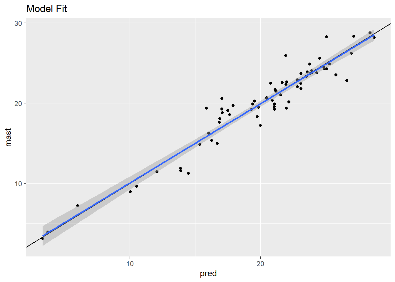
4.6.4 Model Interpretation
A nice feature of linear models are that they are easy to interpret. If we examine the model coefficients we can see how what we’re trying to predict (i.e. the response variable) varies as a function of the GIS variables (i.e. predictor variables). So looking at the elev variable below we can see that mast decreasing at a rate of -0.066 for every change in elevation.
## Linear Regression Model
##
## ols(formula = mast ~ elev + solarcv + tc_1 + tc_2, data = data,
##     weights = data$numDays, x = TRUE, y = TRUE)
##
##                  Model Likelihood    Discrimination
##                        Ratio Test           Indexes
## Obs       68    LR chi2    177.01    R2       0.926
## sigma73.3628    d.f.            4    R2 adj   0.921
## d.f.      63    Pr(> chi2) 0.0000    g        5.720
##
## Residuals
##
##     Min      1Q  Median      3Q     Max
## -3.7912 -0.8006 -0.1218  0.7401  4.0016
##
##
##           Coef    S.E.   t      Pr(>|t|)
## Intercept 49.9906 3.7439  13.35 <0.0001
## elev      -0.0066 0.0006 -11.82 <0.0001
## solarcv   -0.2421 0.0526  -4.60 <0.0001
## tc_1      -0.0535 0.0113  -4.75 <0.0001
## tc_2 -0.1469 0.0362 -4.06 0.0001We can examine how much each variable contributes to the model by examining the results of anova. From the summary below we can that the majority of partial sum of squares are captured by elev, with progressively less by the remaining variables.
##                 Analysis of Variance          Response: mast
##
##  Factor     d.f. Partial SS MS          F      P
##  elev        1    751577.78  751577.776 139.64 <.0001
##  solarcv     1    114017.66  114017.655  21.18 <.0001
##  tc_1        1    121686.11  121686.110  22.61 <.0001
##  tc_2        1     88784.39   88784.388  16.50 1e-04
##  REGRESSION  4   4240328.96 1060082.241 196.96 <.0001
##  ERROR      63    339072.21    5382.099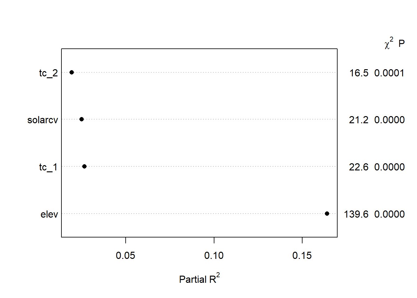
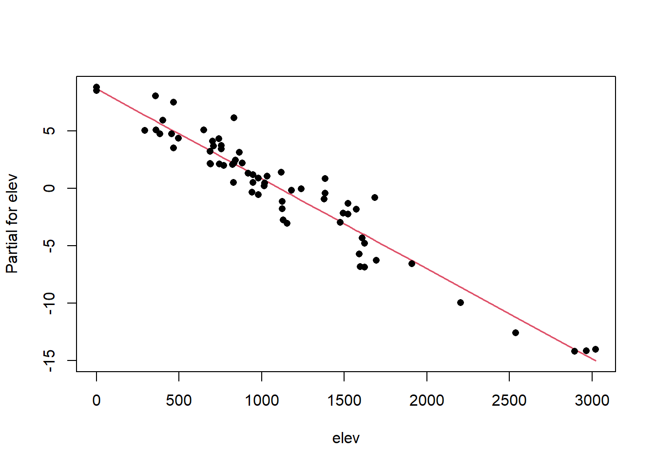
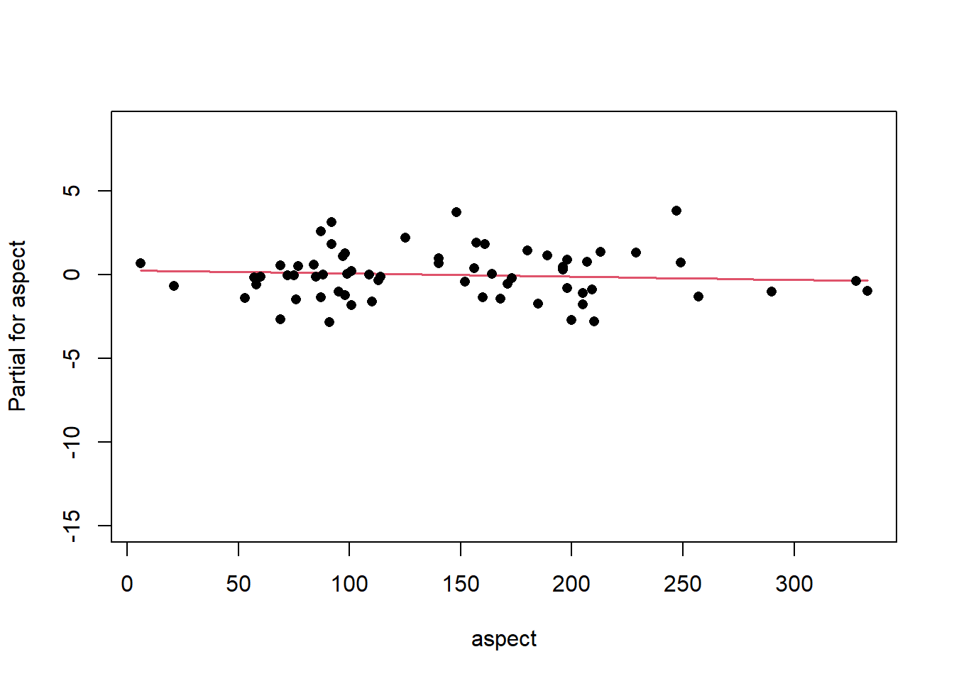
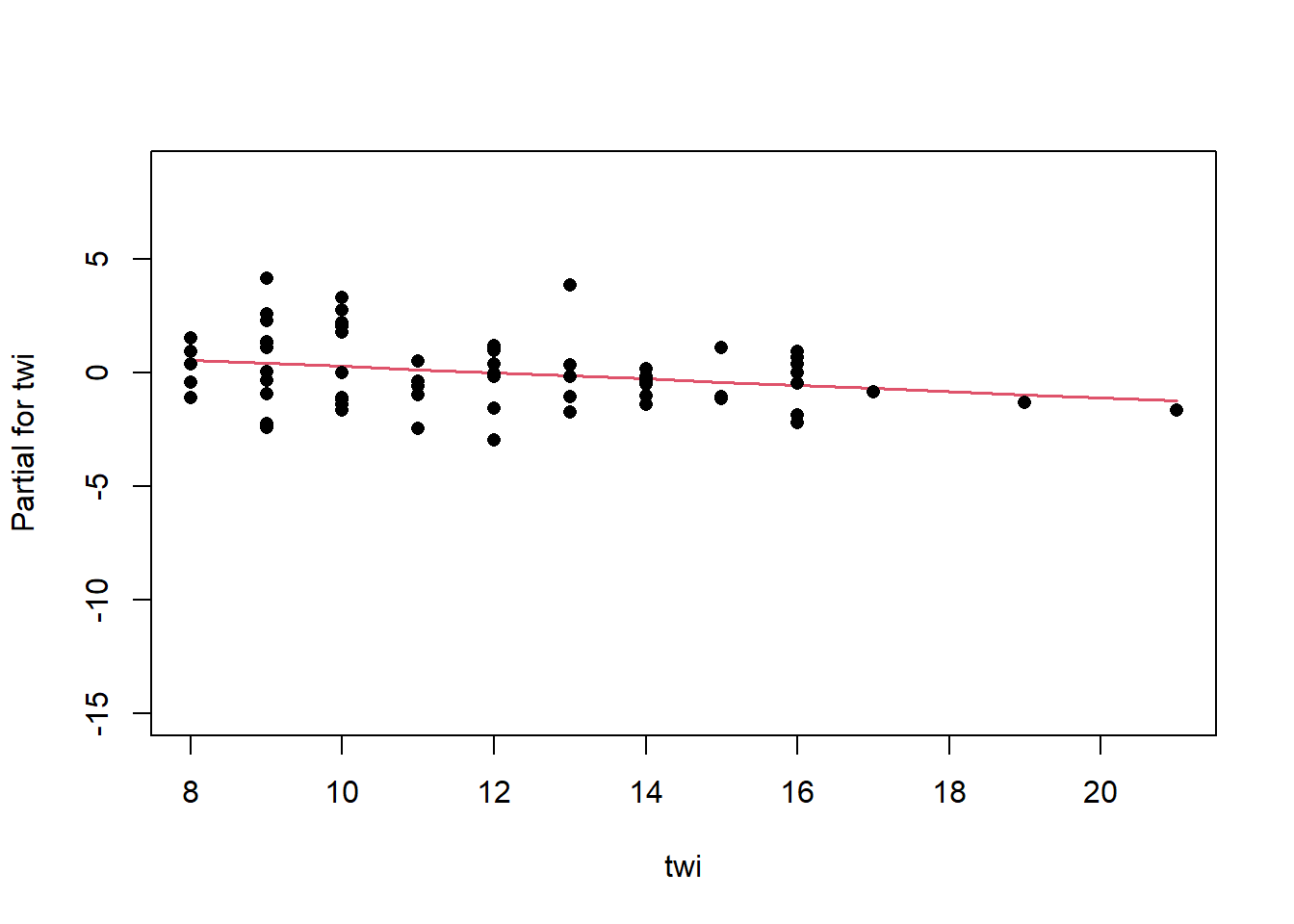
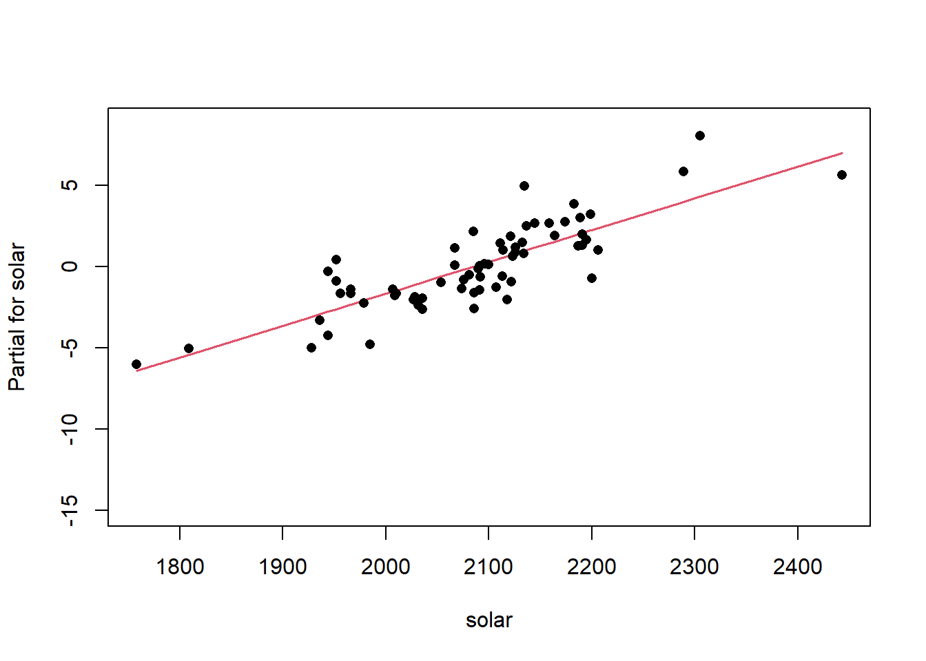
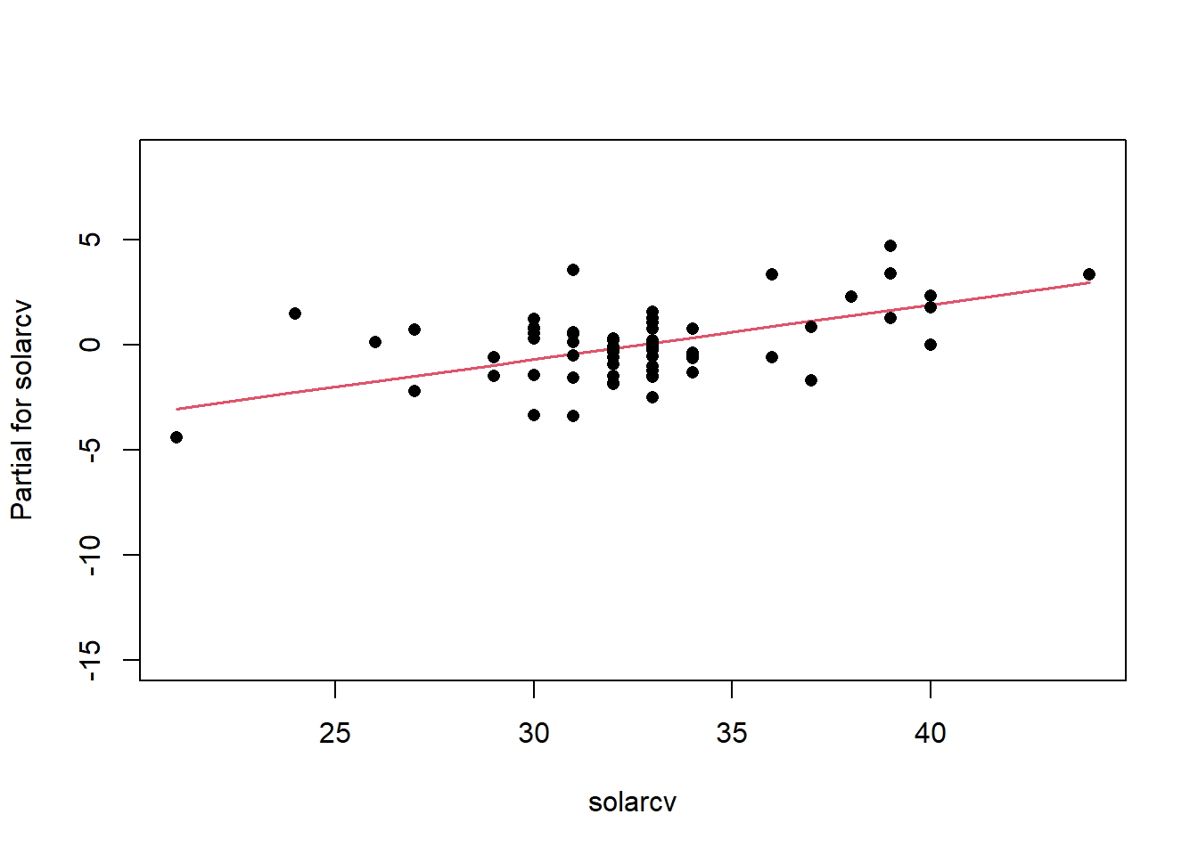
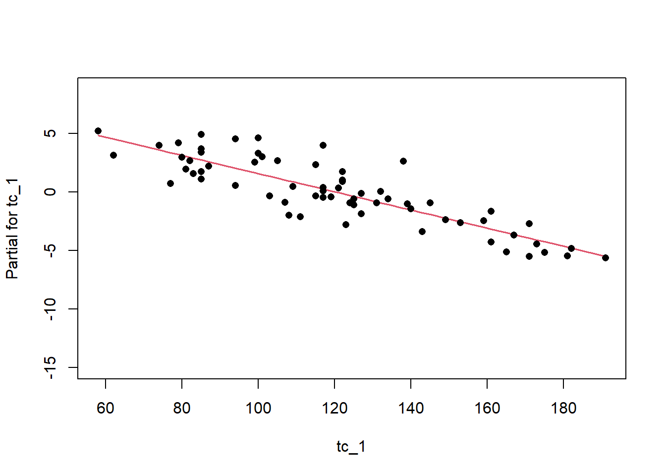
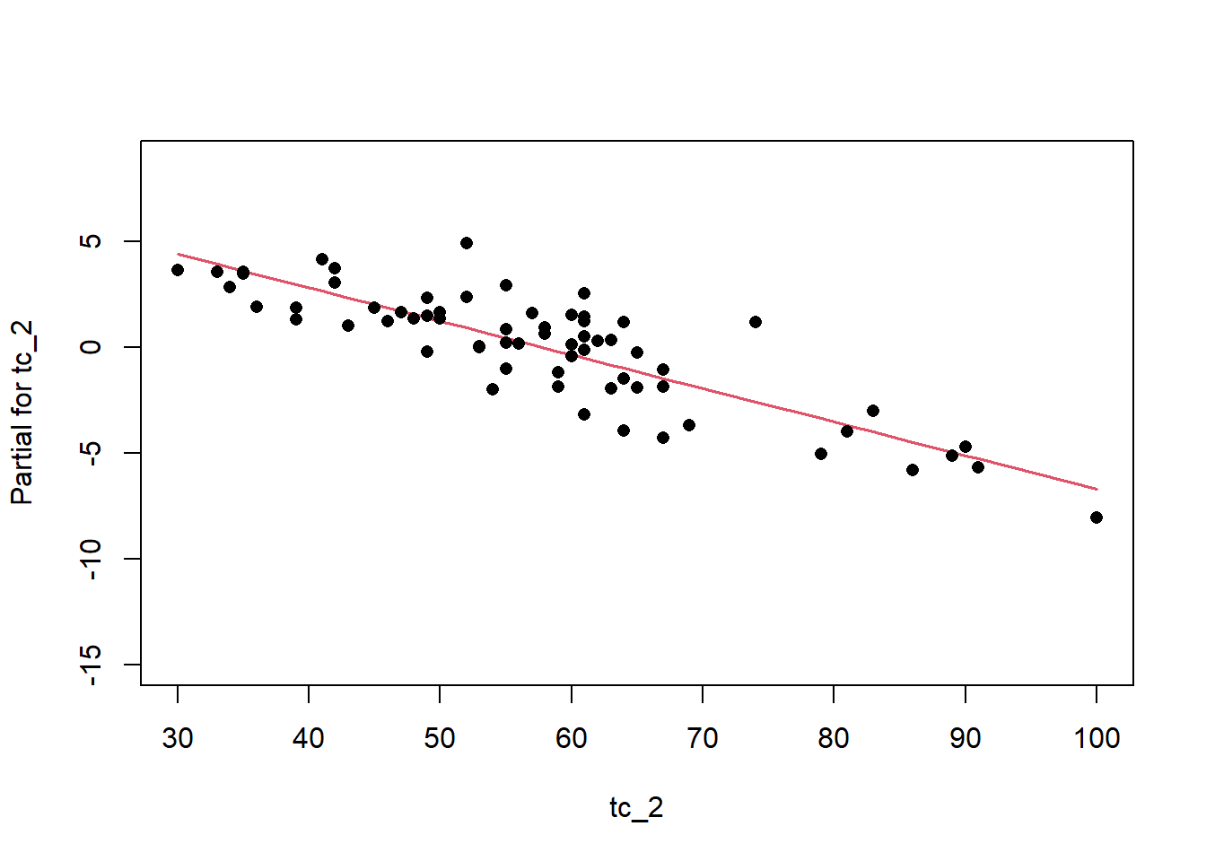
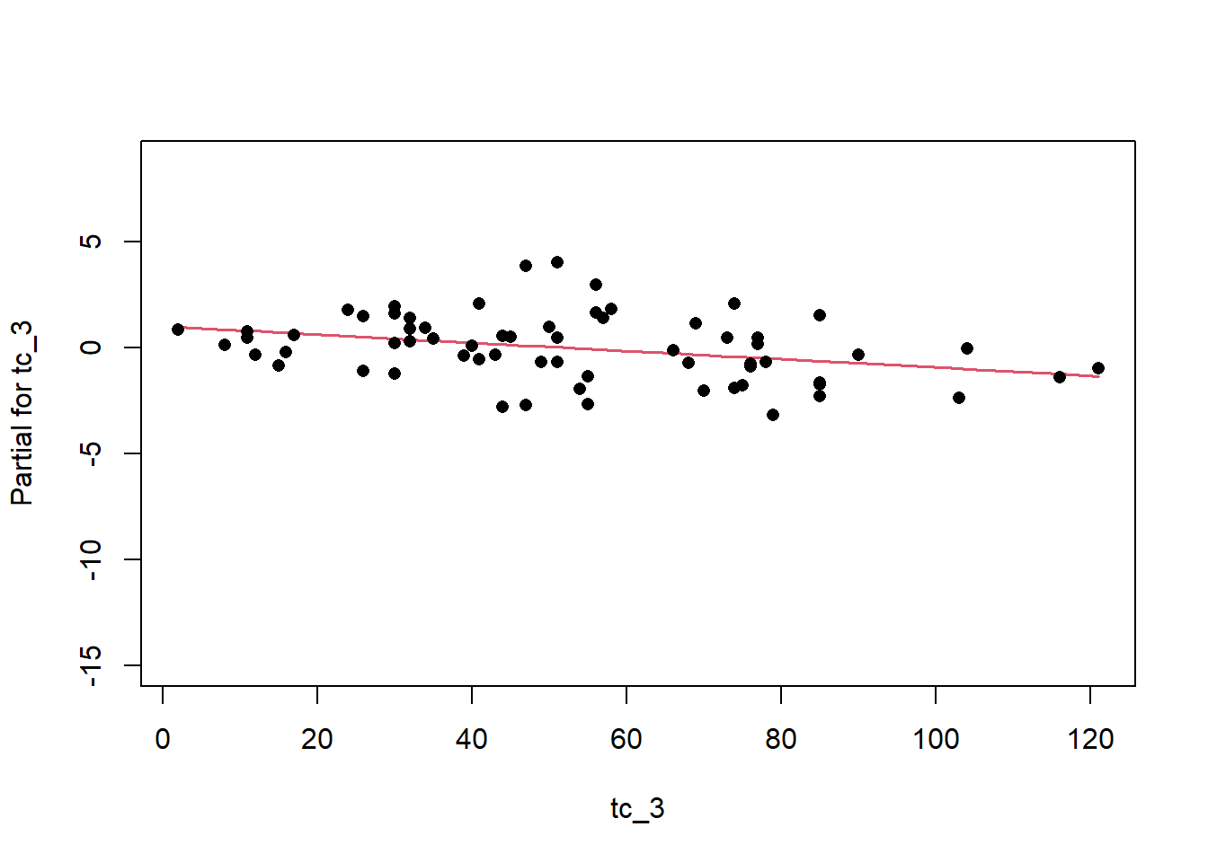
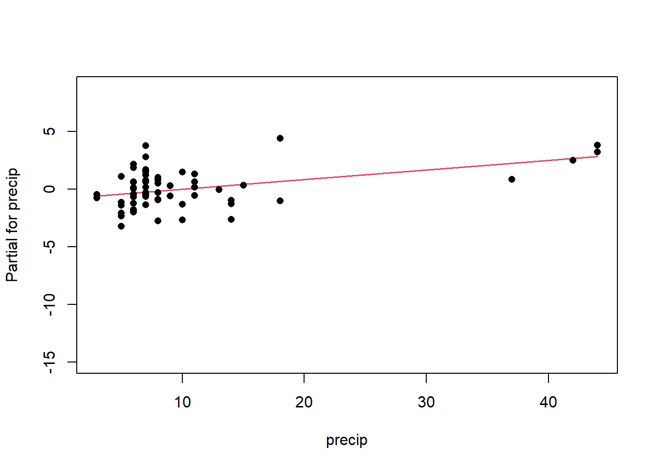
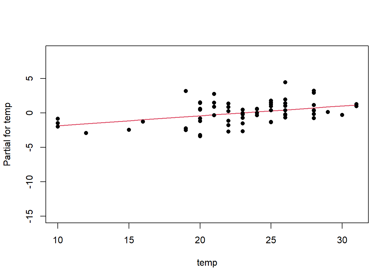
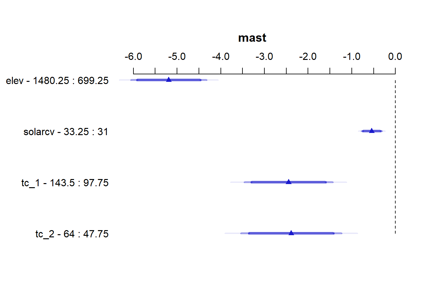
Another way to visualize the contribution of each variable is to plot their partial effects, which summarize how much each variable effects the model if we hold all the other variables constant at their median values and vary the variable of interest over it’s 25th and 75th percentiles. This is a useful way to compare the impact of each variable side by side in the units of the response variable. In this case we can see below that again elev has the biggest impact, with range of approximately -6 to -4.5 degrees. The effect of solarcv is smallest compared to the other tasseled cap variables.
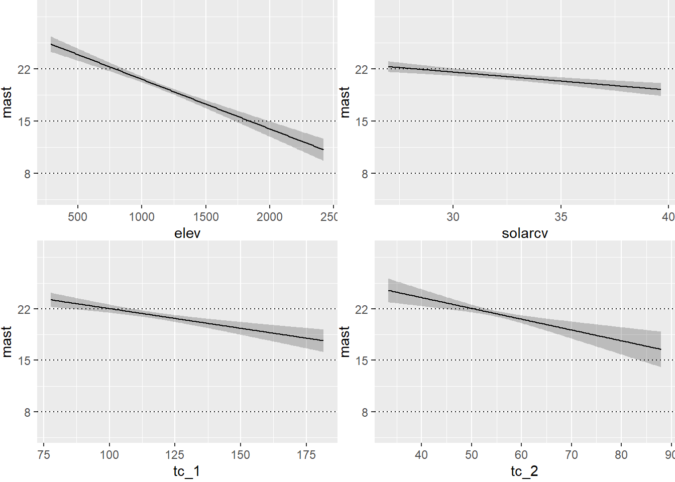
The partial effects can also be visualized as regression lines with their confidence intervals, which illustrates the slope of the predictor variables in relation to mast.
# Plot Effects
ggplot(Predict(final_ols),
       addlayer = geom_hline(yintercept = c(8, 15, 22), linetype = "dotted") +
         scale_y_continuous(breaks = c(8, 15, 22))
       )
# Vary solarcv (North = 23; Flat = 33; South = 55)
ggplot(Predict(final_ols, elev = NA, solarcv = c(23, 33, 51))) +
  geom_hline(yintercept = c(8, 15, 22), linetype = "dotted") +
  scale_y_continuous(breaks = c(8, 15, 22))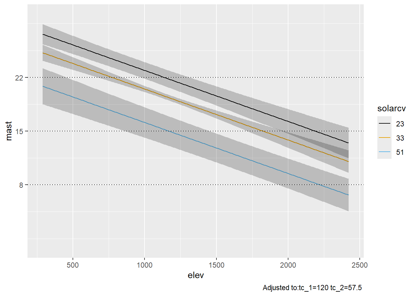
4.9 Exercise
- Load the CA790 MAST dataset.
url <- "https://raw.githubusercontent.com/ncss-tech/stats_for_soil_survey/master/exercises/yosemite-example/henry_CA790_data.csv"
mast2 <- read.csv(url)
Fit a linear model.
Examine the residuals and check for multi-collinearity.
- Are their any outliers?
Perform a variable selection.
- Does the automatic selection make sense?
Assess the model accuracy and plot the fit.
- How do the train vs test accuracies compare?
Summarize and plot the model effects.
- Which variable has the steepest slope?
- Which variable has the greatest effect?
- Which variable explains the most variance?
4.10 Additional reading
The proper use and misuse of regression in soil science has been described by (Webster 1997). James et al. (2021) provide a useful introduction to linear regression. For more discussion of extending regression to incorporate spatial trends in the residuals see Hengl (2009).
Frank Harrel’s Regression Modeling Strategies book and website offer detailed commentary on the entire process of selecting an appropriate model form, model calibration, model validation, and interpretation.