Mapping Dominant Ecological Sites using SSURGO Data
Source:vignettes/dominant-es.Rmd
dominant-es.RmdOverview
This vignette demonstrates how to extract and map dominant ecological
site information for a given Area of Interest (AOI) using the
soilDB package and open-source geospatial tools in R.
For a general introduction to geospatial data in R, see the sf package
documentation, terra package
documentation, the Geocomputation with R book
and the Spatial Data Science with R
and terra book.
We will:
Load SSURGO spatial data
Query Soil Data Access (SDA) for dominant ecological site assignments
Join tabular and spatial data
Export and visualize the results
Prerequisites
In this vignette we will use sf functions and object
types for processing and storing spatial data. This package is used
under the hood by soilDB for processing SSURGO data. The
terra package can be used with only minor changes in
syntax.
Load SSURGO Spatial Data
Using Soil Data Access
You can use SDA_spatialQuery() and
fetchSDA_spatial() to retrieve spatial data directly from
Soil Data Access (SDA), bypassing the need for local files.
Option 1: Use SDA_spatialQuery() to get mukey polygons
for an AOI
Define Area of Interest (AOI) as a bounding box sf
POLYGON.
aoi <- sf::st_as_sfc(sf::st_bbox(c(
xmin = -120.85,
xmax = -120.775,
ymin = 37.975,
ymax = 38.0
), crs = 4326))
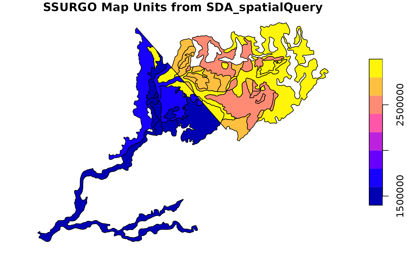
# Query SDA for map unit polygons cropped to the AOI
soil_polygons <- SDA_spatialQuery(
aoi,
what = "mupolygon"
)
plot(
soil_polygons["mukey"],
main = "SSURGO Map Units from SDA_spatialQuery"
)
head(soil_polygons)## Simple feature collection with 6 features and 2 fields
## Geometry type: POLYGON
## Dimension: XY
## Bounding box: xmin: -120.8235 ymin: 37.98283 xmax: -120.7807 ymax: 38.01469
## Geodetic CRS: WGS 84
## mukey area_ac geom
## 1 2441798 187.863380 POLYGON ((-120.7961 38.0051...
## 2 2924886 6.788244 POLYGON ((-120.8201 37.9839...
## 3 2450844 30.732837 POLYGON ((-120.7897 37.9864...
## 4 2924752 11.813110 POLYGON ((-120.7836 37.9887...
## 5 2441798 32.166563 POLYGON ((-120.7884 37.9883...
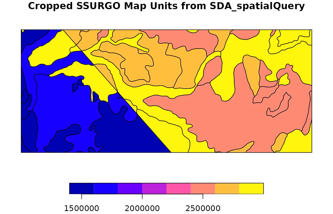
## 6 2450844 48.484422 POLYGON ((-120.7985 37.9945...You can also set geomIntersection = TRUE so that
intersecting geometries are cropped to the AOI. This is convenient if
you have a very specific AOI in mind or would like to reduce the amount
of data you are going to download.
# Query SDA for map unit polygons cropped to the AOI
soil_polygons <- SDA_spatialQuery(
  aoi,
  what = "mupolygon",
  geomIntersection = TRUE
)

plot(
  soil_polygons["mukey"],
  main = "Cropped SSURGO Map Units from SDA_spatialQuery"
)
head(soil_polygons)## Simple feature collection with 6 features and 2 fields
## Geometry type: POLYGON
## Dimension: XY
## Bounding box: xmin: -120.8235 ymin: 37.98283 xmax: -120.7807 ymax: 38
## Geodetic CRS: WGS 84
## mukey area_ac geom
## 1 2441798 26.735794 POLYGON ((-120.7922 37.998,...
## 2 2924886 6.788244 POLYGON ((-120.82 37.98283,...
## 3 2450844 30.732837 POLYGON ((-120.79 37.98505,...
## 4 2924752 11.813110 POLYGON ((-120.7836 37.9887...
## 5 2441798 32.166563 POLYGON ((-120.786 37.98831...
## 6 2450844 48.484422 POLYGON ((-120.8046 37.9885...Option 2: Use fetchSDA_spatial()
Next, we use fetchSDA_spatial().
This function is different because instead of using an area of interest, it takes a vector of map unit or legend identifiers.
Here, we take the unique map unit keys from the Option 1 result and return the full extent of those map units (not just the intersecting polygons). This is particularly helpful when doing studies that involve the full extent of map unit concepts, as opposed to more site-specific analyses.
mu_ssurgo <- fetchSDA_spatial(
  unique(soil_polygons$mukey),
  by.col = "mukey",
  add.fields = c("legend.areaname",
                 "mapunit.muname",
                 "mapunit.farmlndcl")
)

plot(mu_ssurgo["mukey"], main = "SSURGO Map Units from fetchSDA_spatial")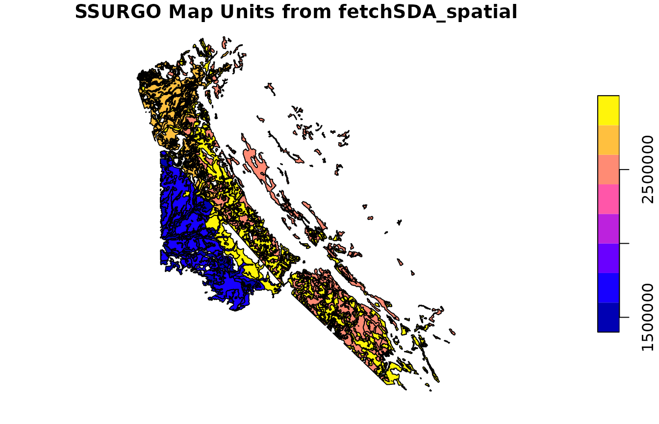
head(mu_ssurgo)## Simple feature collection with 6 features and 6 fields
## Geometry type: POLYGON
## Dimension: XY
## Bounding box: xmin: -120.8318 ymin: 37.87806 xmax: -120.6511 ymax: 38.09373
## Geodetic CRS: WGS 84
## mukey areasymbol nationalmusym
## 1 2441798 CA630 2mywp
## 2 2441798 CA630 2mywp
## 3 2441798 CA630 2mywp
## 4 2441798 CA630 2mywp
## 5 2441798 CA630 2mywp
## 6 2441798 CA630 2mywp
## areaname
## 1 Central Sierra Foothills Area, California, Parts of Calaveras and Tuolumne Counties
## 2 Central Sierra Foothills Area, California, Parts of Calaveras and Tuolumne Counties
## 3 Central Sierra Foothills Area, California, Parts of Calaveras and Tuolumne Counties
## 4 Central Sierra Foothills Area, California, Parts of Calaveras and Tuolumne Counties
## 5 Central Sierra Foothills Area, California, Parts of Calaveras and Tuolumne Counties
## 6 Central Sierra Foothills Area, California, Parts of Calaveras and Tuolumne Counties
## muname farmlndcl
## 1 Bonanza-Loafercreek complex, 3 to 15 percent slopes Not prime farmland
## 2 Bonanza-Loafercreek complex, 3 to 15 percent slopes Not prime farmland
## 3 Bonanza-Loafercreek complex, 3 to 15 percent slopes Not prime farmland
## 4 Bonanza-Loafercreek complex, 3 to 15 percent slopes Not prime farmland
## 5 Bonanza-Loafercreek complex, 3 to 15 percent slopes Not prime farmland
## 6 Bonanza-Loafercreek complex, 3 to 15 percent slopes Not prime farmland
## geom
## 1 POLYGON ((-120.6513 37.9647...
## 2 POLYGON ((-120.7555 37.9478...
## 3 POLYGON ((-120.7659 38.0160...
## 4 POLYGON ((-120.7961 38.0051...
## 5 POLYGON ((-120.8276 38.0924...
## 6 POLYGON ((-120.7017 37.8785...Note that using add.fields we have included some
additional contextual information: area name, map unit name, and map
unit farmland classification.
fetchSDA_spatial() geometry sources
fetchSDA_spatial() geom.src argument can be
used to return SSURGO map unit polygons and survey area polygons,
STATSGO mapunit polygons, and MLRA polygons.
Here is an example using STATSGO. We use
SDA_spatialQuery() to fetch the data for our AOI, then
fetchSDA_spatial() to get the full extent of those map unit
concepts.
statsgo_polygons <- SDA_spatialQuery(
  aoi,
  what = "mupolygon",
  db = "STATSGO",
  geomIntersection = TRUE
)

plot(statsgo_polygons["mukey"], main = "STATSGO Map Units from SDA_spatialQuery")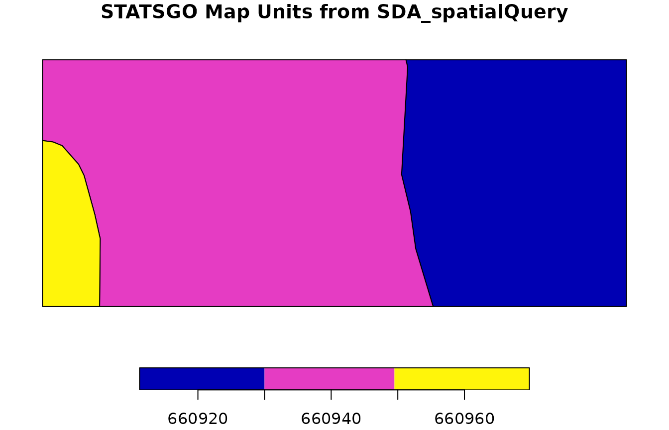
head(statsgo_polygons)## Simple feature collection with 3 features and 2 fields
## Geometry type: POLYGON
## Dimension: XY
## Bounding box: xmin: -120.85 ymin: 37.975 xmax: -120.775 ymax: 38
## Geodetic CRS: WGS 84
## mukey area_ac geom
## 1 660921 1668.6742 POLYGON ((-120.7998 37.975,...
## 2 660939 2596.0225 POLYGON ((-120.8427 37.975,...
## 3 660960 253.0798 POLYGON ((-120.85 37.975, -...
mu_statsgo <- fetchSDA_spatial(
  unique(statsgo_polygons$mukey),
  by.col = "mukey",
  db = "STATSGO",
  add.fields = c("legend.areaname", "mapunit.muname", "mapunit.farmlndcl")
)

plot(mu_statsgo["mukey"], main = "STATSGO Map Units from fetchSDA_spatial")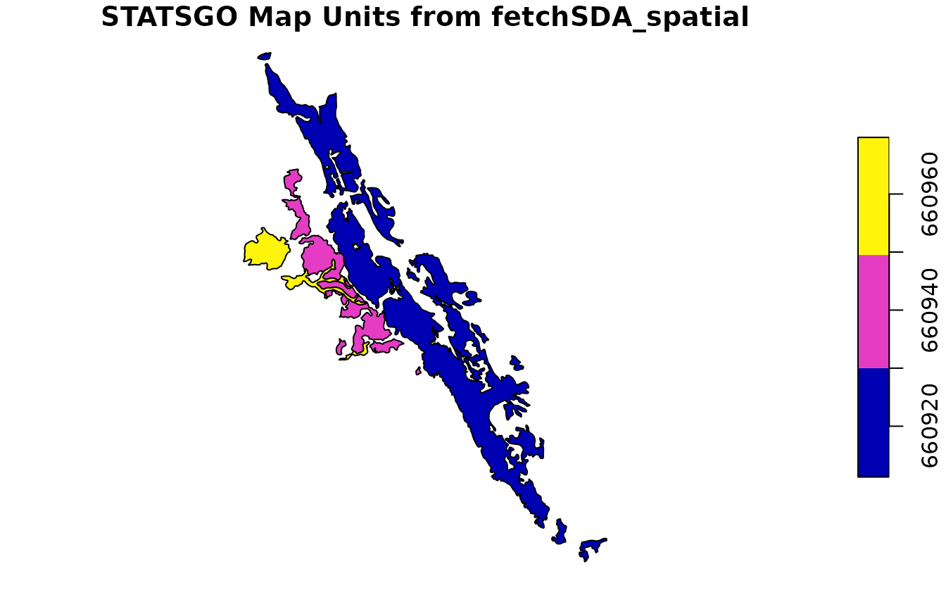
head(mu_statsgo)## Simple feature collection with 6 features and 6 fields
## Geometry type: POLYGON
## Dimension: XY
## Bounding box: xmin: -121.2368 ymin: 37.07511 xmax: -119.9157 ymax: 38.18986
## Geodetic CRS: WGS 84
## mukey areasymbol nationalmusym areaname
## 1 660921 US q5r1 United States
## 2 660939 US q5rm United States
## 3 660960 US q5s9 United States
## 4 660960 US q5s9 United States
## 5 660960 US q5s9 United States
## 6 660939 US q5rm United States
## muname farmlndcl geom
## 1 Whiterock-Rock outcrop-Auburn (s818) <NA> POLYGON ((-120.794 38.18986...
## 2 Peters-Pentz (s836) <NA> POLYGON ((-120.9141 38.0735...
## 3 Finrod-Cogna-Archerdale (s857) <NA> POLYGON ((-120.9711 37.9490...
## 4 Finrod-Cogna-Archerdale (s857) <NA> POLYGON ((-120.7151 37.7056...
## 5 Finrod-Cogna-Archerdale (s857) <NA> POLYGON ((-121.1592 38.0989...
## 6 Peters-Pentz (s836) <NA> POLYGON ((-120.8224 37.7205...
ssas <- SDA_spatialQuery(aoi, what = "areasymbol")
ssas
## areasymbol
## 1 CA630
## 2 CA632
ssa <- fetchSDA_spatial(
  ssas$areasymbol,
  by.col = "areasymbol",
  geom.src = "sapolygon",
  add.fields = c("legend.areaname")
)

plot(ssa["areasymbol"], main = "SSURGO Soil Survey Area from SDA")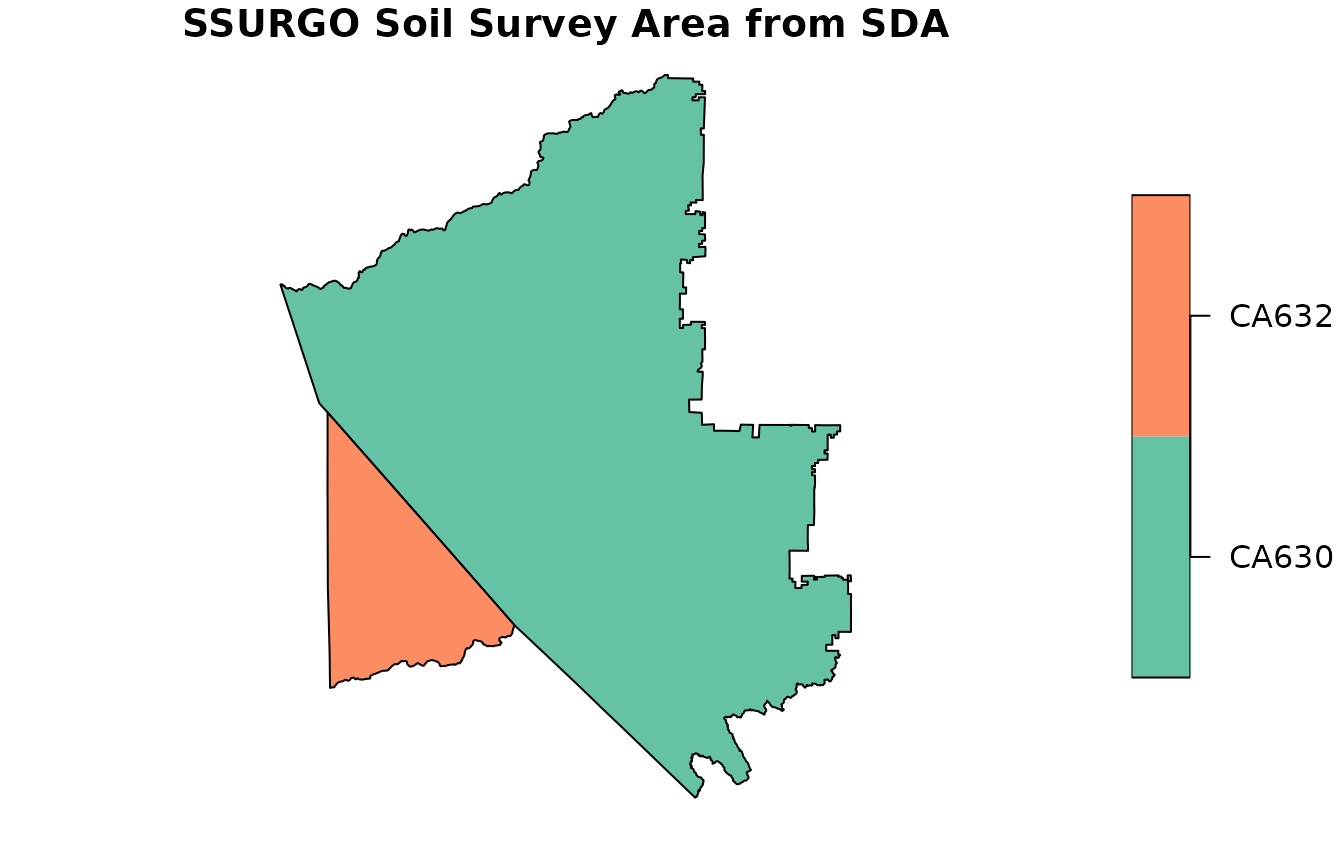
head(ssa)## Simple feature collection with 2 features and 3 fields
## Geometry type: POLYGON
## Dimension: XY
## Bounding box: xmin: -120.9955 ymin: 37.63352 xmax: -120.1595 ymax: 38.46714
## Geodetic CRS: WGS 84
## lkey areasymbol
## 1 14103 CA630
## 2 17969 CA632
## areaname
## 1 Central Sierra Foothills Area, California, Parts of Calaveras and Tuolumne Counties
## 2 Stanislaus County, California, Northern Part
## geom
## 1 POLYGON ((-120.3907 38.4630...
## 2 POLYGON ((-120.6584 37.8202...
SDA_spatialQuery()
vs. fetchSDA_spatial()
SDA_spatialQuery()is ideal for spatial queries where you have a specific, possibly complex, area of interest.fetchSDA_spatial()returns the full extent of the specified map unit concepts, optionally including more legend and map unit attributes viaadd.fieldsargument.
Local Data Sources
If working with large extents, it is generally better to be use a
local data source. You can download SSURGO data from Web Soil Survey
using downloadSSURGO(). Then, you can create GeoPackage or
other database types using createSSURGO() or the SSURGOPortal
tools. This process is described in detail in the Local
SSURGO Databases vignette. See also the SSURGOPortal R
package.
Assuming you have a GeoPackage from SSURGOPortal
("soilmu_a.gpkg"), then you can read it with
sf::st_read() or terra::vect()
ssurgo_path <- "data/soilmu_a.gpkg"  # Replace with your actual path
soil_polygons <- sf::st_read(ssurgo_path)
head(soil_polygons)
This soil_polygons object should have the standard set
of columns we would expect for a SSURGO map unit data source, including:
map unit key (mukey), area symbol
(areasymbol), map unit symbol (musym).
Query SDA for Dominant Ecological Site Info
Extract Unique Map Unit Keys
As we did above for fetchSDA_spatial() we are going to
get the unique set of map units in our AOI.
mukeys <- unique(soil_polygons$mukey)Use get_SDA_coecoclass()
eco_data <- get_SDA_coecoclass(mukeys = mukeys)
head(eco_data)
## mukey areasymbol lkey muname cokey
## 1 1403409 CA632 17969 Archerdale clay loam, 0 to 2 percent slopes 27449761
## 2 1403409 CA632 17969 Archerdale clay loam, 0 to 2 percent slopes 27449762
## 3 1403409 CA632 17969 Archerdale clay loam, 0 to 2 percent slopes 27449763
## 4 1403409 CA632 17969 Archerdale clay loam, 0 to 2 percent slopes 27449764
## 5 1403409 CA632 17969 Archerdale clay loam, 0 to 2 percent slopes 27449765
## 6 1403409 CA632 17969 Archerdale clay loam, 0 to 2 percent slopes 27449766
## coecoclasskey comppct_r majcompflag compname localphase compkind
## 1 NA 4 No Capay clay Series
## 2 NA 1 No Chuloak sandy loam Series
## 3 NA 2 No Clear Lake clay Series
## 4 NA 1 No Finrod clay Series
## 5 NA 3 No Hicksville loam Series
## 6 NA 3 No Hollenbeck clay Series
## ecoclassid ecoclassname ecoclasstypename ecoclassref
## 1 Not assigned Not assigned Not assigned Not assigned
## 2 Not assigned Not assigned Not assigned Not assigned
## 3 Not assigned Not assigned Not assigned Not assigned
## 4 Not assigned Not assigned Not assigned Not assigned
## 5 Not assigned Not assigned Not assigned Not assigned
## 6 Not assigned Not assigned Not assigned Not assignedThis function returns a data frame including mukey,
cokey, ecoclassid, and
ecoclassname.
There are several methods for aggregating from component to map unit
level available in get_SDA_coecoclass(). The default
aggregation method is "none" which will return 1 record per
map unit component, so many map units will have more than one
record.
Using method="dominant component"
Most often, users want “typical” conditions that can apply to a whole map unit.
Sometimes it is helpful to be able to point to a specific
component, so that you do not have to reason over mathematical
aggregation of distinct components within map unit concepts. The most
common method to select one component per map unit is
"dominant component"
eco_data_domcond <- get_SDA_coecoclass(
  mukeys = mukeys,
  method = "dominant component"
)
head(eco_data_domcond)
## mukey areasymbol lkey
## 8 1403409 CA632 17969
## 13 1403418 CA632 17969
## 15 1403432 CA632 17969
## 19 1403439 CA632 17969
## 30 1540892 CA632 17969
## 31 1605509 CA632 17969
## muname cokey
## 8 Archerdale clay loam, 0 to 2 percent slopes 27449768
## 13 Hicksville loam, 0 to 2 percent slopes, occasionally flooded 27449813
## 15 Redding gravelly loam, 0 to 8 percent slopes, dry 27449968
## 19 Peters-Pentz association, 2 to 8 percent slopes 27450031
## 30 Mckeonhills clay, 5 to 15 percent slopes 27450072
## 31 Pentz-Peters association, 2 to 50 percent slopes 27450044
## coecoclasskey comppct_r majcompflag compname localphase compkind
## 8 12784144 85 Yes Archerdale clay loam Series
## 13 12784163 85 Yes Hicksville loam Series
## 15 12784219 85 Yes Redding gravelly loam Series
## 19 12784259 60 Yes Peters silty clay loam Series
## 30 12784278 90 Yes Mckeonhills clay Series
## 31 12784267 62 Yes Pentz silt loam Series
## ecoclassid ecoclassname ecoclasstypename
## 8 R017XY903CA Stream Channels and Floodplains NRCS Rangeland Site
## 13 R017XY905CA Dry Alluvial Fans and Terraces NRCS Rangeland Site
## 15 R017XY902CA Duripan Vernal Pools NRCS Rangeland Site
## 19 R018XI164CA Clayey Dissected Swales NRCS Rangeland Site
## 30 R018XI163CA Thermic Low Rolling Hills NRCS Rangeland Site
## 31 R018XI163CA Thermic Low Rolling Hills NRCS Rangeland Site
## ecoclassref
## 8 Ecological Site Description Database
## 13 Ecological Site Description Database
## 15 Ecological Site Description Database
## 19 Ecological Site Description Database
## 30 Ecological Site Description Database
## 31 Ecological Site Description DatabaseNote that this output includes information for the dominant component
(comppct_r and compname).
Using method="dominant condition"
The method "dominant condition" is convenient because it
accounts for the possibility that multiple components have the same
class (ecological site) and can have their component percentages
summed.
For a property like ecological site, it is fairly common for multiple components in a map unit to have the same site assigned, so the dominant condition makes up a higher percentage of the area of the map unit than the dominant component alone.
eco_data_domcond <- get_SDA_coecoclass(
  mukeys = mukeys,
  method = "dominant condition"
)
head(eco_data_domcond)
## mukey areasymbol lkey
## 8 1403409 CA632 17969
## 13 1403418 CA632 17969
## 15 1403432 CA632 17969
## 19 1403439 CA632 17969
## 30 1540892 CA632 17969
## 31 1605509 CA632 17969
## muname cokey
## 8 Archerdale clay loam, 0 to 2 percent slopes 27449768
## 13 Hicksville loam, 0 to 2 percent slopes, occasionally flooded 27449813
## 15 Redding gravelly loam, 0 to 8 percent slopes, dry 27449968
## 19 Peters-Pentz association, 2 to 8 percent slopes 27450031
## 30 Mckeonhills clay, 5 to 15 percent slopes 27450072
## 31 Pentz-Peters association, 2 to 50 percent slopes 27450044
## coecoclasskey comppct_r majcompflag compname localphase compkind
## 8 12784144 85 Yes Archerdale clay loam Series
## 13 12784163 85 Yes Hicksville loam Series
## 15 12784219 85 Yes Redding gravelly loam Series
## 19 12784259 60 Yes Peters silty clay loam Series
## 30 12784278 90 Yes Mckeonhills clay Series
## 31 12784267 62 Yes Pentz silt loam Series
## ecoclassid ecoclassname ecoclasstypename
## 8 R017XY903CA Stream Channels and Floodplains NRCS Rangeland Site
## 13 R017XY905CA Dry Alluvial Fans and Terraces NRCS Rangeland Site
## 15 R017XY902CA Duripan Vernal Pools NRCS Rangeland Site
## 19 R018XI164CA Clayey Dissected Swales NRCS Rangeland Site
## 30 R018XI163CA Thermic Low Rolling Hills NRCS Rangeland Site
## 31 R018XI163CA Thermic Low Rolling Hills NRCS Rangeland Site
## ecoclassref ecoclasspct_r
## 8 Ecological Site Description Database 85
## 13 Ecological Site Description Database 85
## 15 Ecological Site Description Database 85
## 19 Ecological Site Description Database 60
## 30 Ecological Site Description Database 92
## 31 Ecological Site Description Database 67Note that this result includes the aggregate ecological site
composition ecoclasspct_r.
The cokey and comppct_r are from the
dominant component can be used to link to a specific, common component
for other more detailed information.
Join Tabular and Spatial Data
We want to have a 1:1 relationship between our map unit polygons and
the thematic variable we are mapping, so we will use the map unit
dominant condition ecological sites (eco_data_domcond).
soil_polygons <- merge(
  soil_polygons,
  eco_data_domcond,
  by = "mukey"
)
Visualize the Result
plot(
  soil_polygons["ecoclassid"],
  main = "Dominant Ecological Site by Map Unit"
)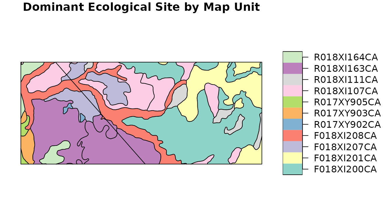
This same process for merging in aggregate map unit level information
generalizes to other SSURGO tables. You can easily create thematic maps
from any data you can aggregate to the point that it is 1:1 with the
mukey.
Export Spatial File
Finally, we can write our result out to a spatial file, such as a
GeoPackage, using sf or terra.
sf::st_write(
  soil_polygons,
  "ecosite_dominant.gpkg",
  delete_dsn = TRUE
)