Plot a component relation graph

Plot a component relation graph based on an adjacency or similarity matrix.

plotSoilRelationGraph(
  m,
  s = "",
  plot.style = c("network", "dendrogram", "none"),
  graph.mode = "upper",
  spanning.tree = NULL,
  del.edges = NULL,
  vertex.scaling.method = "degree",
  vertex.scaling.factor = 2,
  edge.scaling.factor = 1,
  vertex.alpha = 0.65,
  edge.transparency = 1,
  edge.col = grey(0.5),
  edge.highlight.col = "royalblue",
  g.layout = igraph::layout_with_fr,
  vertex.label.color = "black",
  delete.singletons = FALSE,
  ...
)

Arguments

m

adjacency matrix

s

central component; an empty character string is interpreted as no central component

plot.style

plot style ('network', or 'dendrogram'), or 'none' for no graphical output

graph.mode

interpretation of adjacency matrix: 'upper' or 'directed', see details

spanning.tree

plot the minimum or maximum spanning tree ('min', 'max'), or, max spanning tree plus edges with weight greater than the n-th quantile specified in spanning.tree. See details and examples.

del.edges

optionally delete edges with weights less than the specified quantile (0-1)

vertex.scaling.method

'degree' (default) or 'distance', see details

vertex.scaling.factor

scaling factor applied to vertex size

edge.scaling.factor

optional scaling factor applied to edge width

vertex.alpha

optional transparency setting for vertices (0-1)

edge.transparency

optional transparency setting for edges (0-1)

edge.col

edge color, applied to all edges

edge.highlight.col

edge color applied to all edges connecting to component named in s

g.layout

an igraph layout function, defaults to igraph::layout_with_fr

vertex.label.color

vertex label color

delete.singletons

optionally delete vertices with no edges (degree == 0)

...

further arguments passed to plotting function

Value

an igraph graph object is invisibly returned

Details

Vertex size is based on a normalized index of connectivity:

• "degree" size = sqrt(igraph::degree(g) / max(igraph::degree(g))) * scaling.factor

• "distance" size = sqrt(igraph::distance(V -> s) / max(igraph::distance(V -> s))) * scaling.factor, where distance(V->s) is the distance from all nodes to the named series, s.

Edge width can be optionally scaled by edge weight by specifying an edge.scaling.factor value. The maximum spanning tree represents a sub-graph where the sum of edge weights are maximized. The minimum spanning tree represents a sub-graph where the sum of edge weights are minimized. The maximum spanning tree is likely a more useful simplification of the full graph, in which only the strongest relationships (e.g. most common co-occurrences) are preserved.

The maximum spanning tree + edges with weights > n-th quantile is an experimental hybrid. The 'backbone' of the graph is created by the maximum spanning tree, and augmented by 'strong' auxiliary edges–defined by a value between 0 and 1.

The graph.mode argument is passed to igraph::graph_from_adjacency_matrix() and determines how vertex relationships are coded in the adjacency matrix m. Typically, the default value of 'upper' (the upper triangle of m contains adjacency information) is the desired mode. If m contains directional information, set graph.mode to 'directed'. This has the side-effect of altering the default community detection algorithm from igraph::cluster_fast_greedy to igraph::cluster_walktrap.

Note

This function is a work in progress, ideas welcome.

Author

D.E. Beaudette

Examples

if (requireNamespace("igraph") && requireNamespace("vegan")) {
  # load sample data set
  data(amador)

  # create weighted adjacency matrix (see ?component.adj.matrix for details)
  m <- component.adj.matrix(amador)

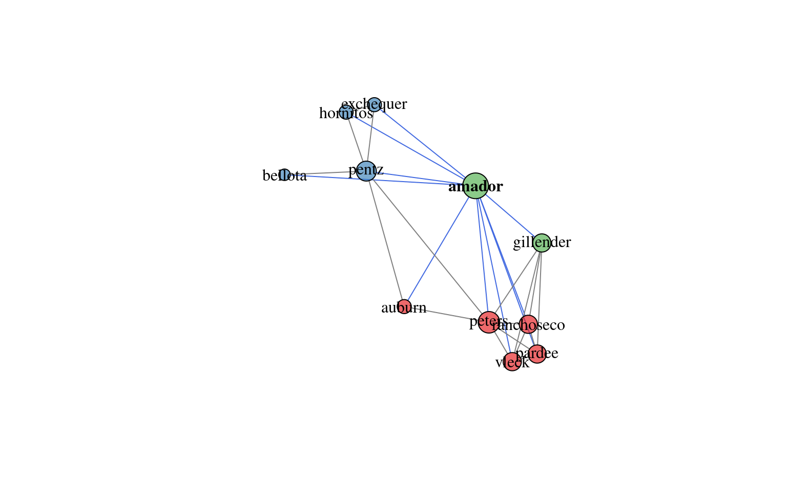
  # plot network diagram, with Amador soil highlighted
  plotSoilRelationGraph(m, s='amador')

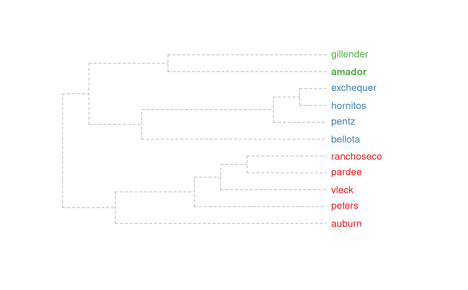
  # dendrogram representation
  plotSoilRelationGraph(m, s='amador', plot.style='dendrogram')

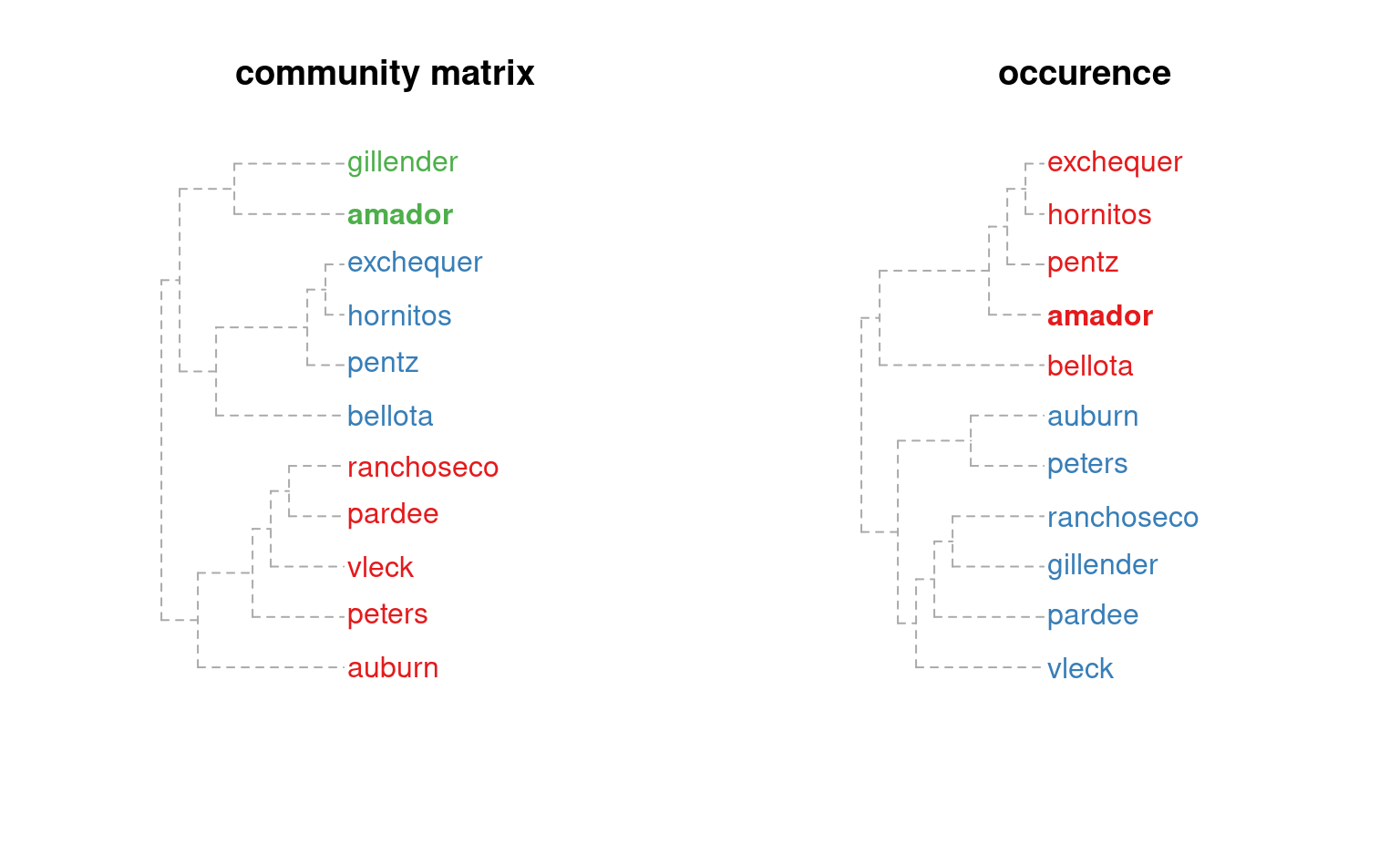
  # compare methods
  m.o <- component.adj.matrix(amador, method='occurrence')

  op <- par(no.readonly = TRUE)

  par(mfcol=c(1,2))
  plotSoilRelationGraph(m, s='amador', plot.style='dendrogram')
  title('community matrix')
  plotSoilRelationGraph(m.o, s='amador', plot.style='dendrogram')
  title('occurence')

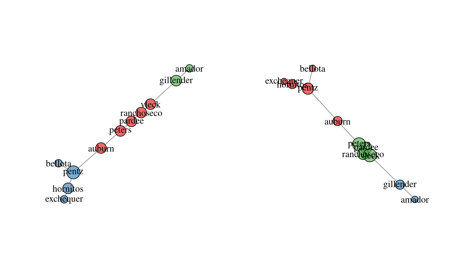
  # investigate max spanning tree
  plotSoilRelationGraph(m, spanning.tree='max')

  # investigate max spanning tree + edges with weights > 75-th pctile
  plotSoilRelationGraph(m, spanning.tree=0.75)

  par(op)

  # \donttest{
  
    if(requireNamespace("curl") &
       curl::has_internet() &
       require(soilDB)) {
    
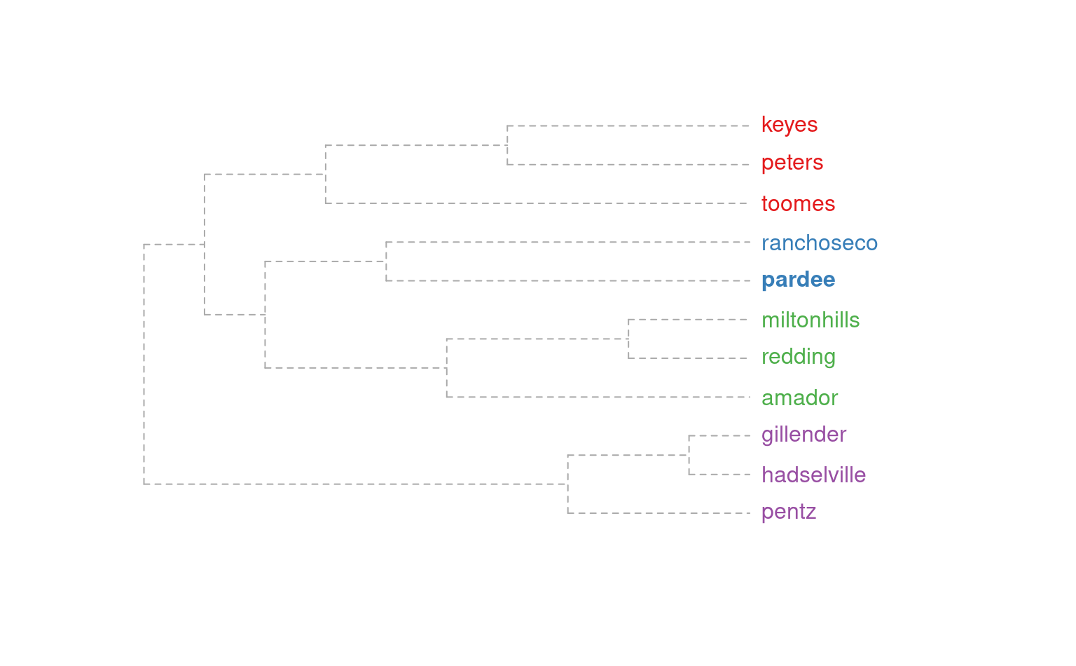
      # get similar data from soilweb, for the Pardee series
      s <- 'pardee'
      d <- siblings(s, component.data = TRUE)
    
      # normalize component names
      d$sib.data$compname <- tolower(d$sib.data$compname)
    
      # keep only major components
      d$sib.data <- subset(d$sib.data, subset=compkind == 'Series')
    
      # build adj. matrix and plot
      m <- component.adj.matrix(d$sib.data)
      plotSoilRelationGraph(m, s=s, plot.style='dendrogram')
    
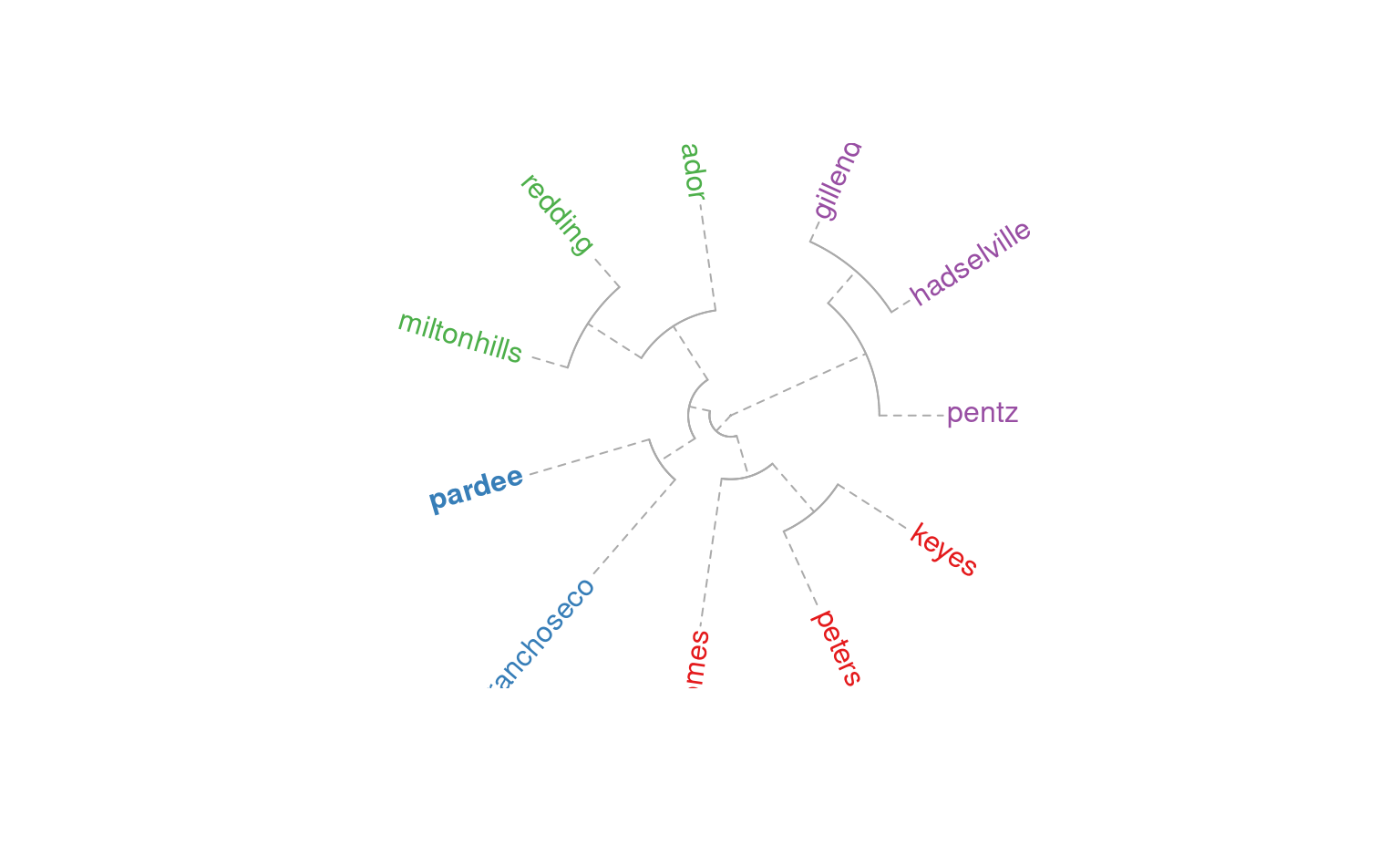
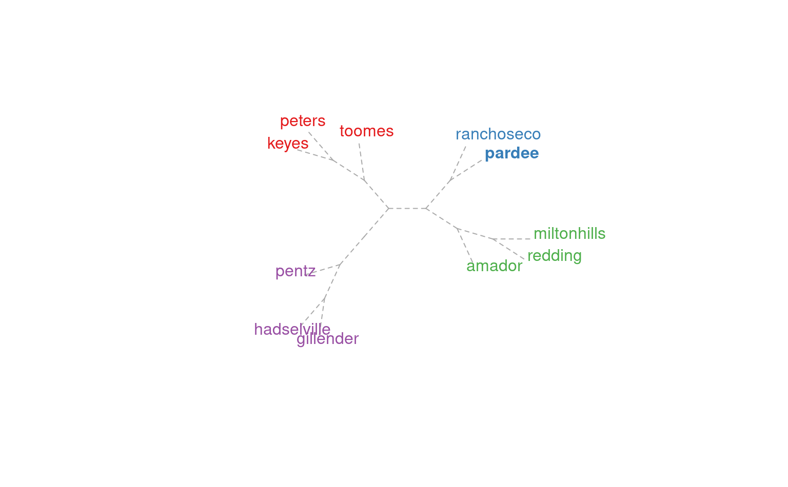
      # alter plotting style, see ?plot.phylo
      plotSoilRelationGraph(m, s=s, plot.style='dendrogram', type='fan')
      plotSoilRelationGraph(m, s=s, plot.style='dendrogram', 
                            type='unrooted', use.edge.length=FALSE) 
    
    }
  # }
}