Applying Newhall to PRISM 30-year Normals for Continental United States • jNSMR

Setup

library(jNSMR)
#> jNSMR (0.3.1) -- R interface to the classic Newhall Simulation Model
#> Added JAR file (newhall-1.6.5.jar) to Java class path.
library(terra)
#> terra 1.7.71

x <- terra::rast(system.file("extdata", "prism_issr800_sample.tif", package = "jNSMR"))
x$elev <- 0 # elevation is not currently used by the model directly

Run simulations

newhall_batch() allows us to provide data in SpatRaster format, and return gridded model results.

# run simulations
y <- newhall_batch(x) ## full resolution
#> newhall_batch: ran n=18790 simulations in 18 secs

Results

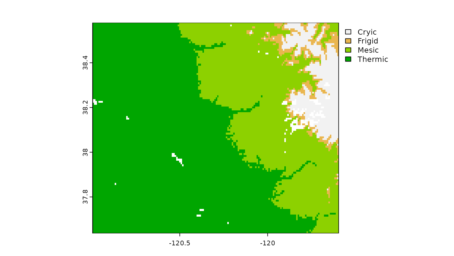
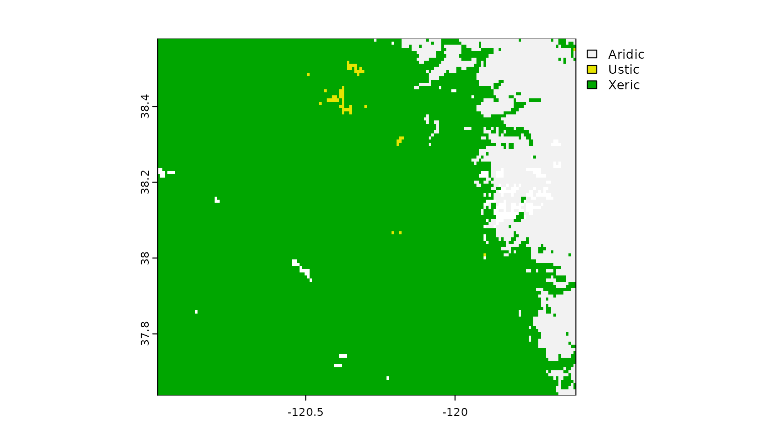
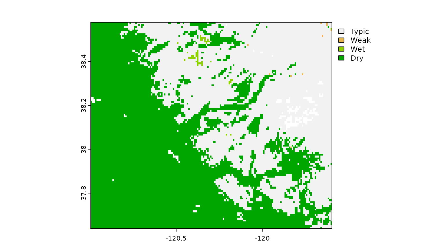
Several categorical quantities are returned related to temperature and moisture regimes, as are a variety of numerical quantities relevant to taxonomic limits and regime criteria.

Temperature Regimes

plot(y$temperatureRegime)

Moisture Regimes

plot(y$moistureRegime)

Moisture Regime Subdivision 1

plot(y$regimeSubdivision1)

Moisture Regime Subdivision 2

plot(y$regimeSubdivision2)

Taxonomic Quantities

panel(y[[c("dryDaysAfterSummerSolstice", "numConsecutiveDaysMoistInSomePartsOver8C")]],
     cex.main = 0.85)

PRISM Data for Custom Extent

The above sample dataset can be easily re-created for arbitrary extents.

First, run the following commands to cache United States (lower 48) PRISM and soil water storage capacity data at 800 meter resolution. In the future there will be options for downloading Alaska, Pacific Islands, Puerto Rico, or any other PRISM data sets.

newhall_prism_cache()
newhall_issr800_cache()

After the above two data sets have been downloaded, combine them and add any other required fields and crop to an extent of interest.

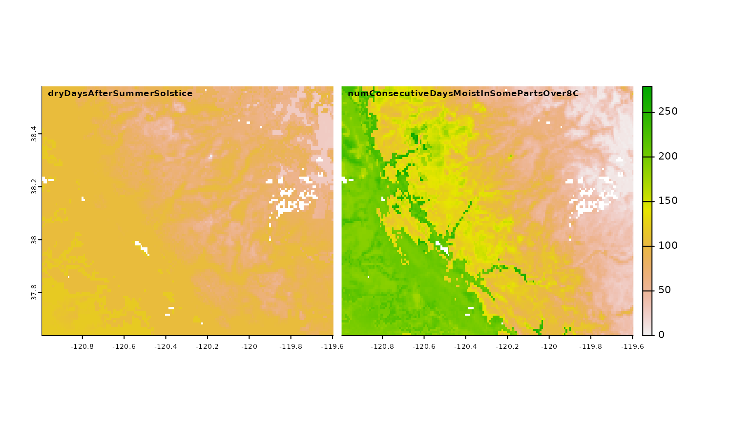
For example, here we use a larger extent aggregated to 8000m resolution to depict a broad transition between the “mesic” and “thermic” temperature regimes.

conus <- c(newhall_prism_rast(), newhall_issr800_rast())
conus$elev <- 0 # elevation is not currently used by the model directly
my_extent <- crop(conus, ext(-91, -88, 37.5, 41.5))

## the above operation can also be achieved with newhall_*_subset() methods
# my_extent <- newhall_prism_subset(ext(-91, -88, 37.5, 41.5))
# my_extent$awc <- newhall_issr800_subset(ext(-91, -88, 37.5, 41.5))
# my_extent$elev <- 0

res <- newhall_batch(aggregate(my_extent, 10, na.rm = TRUE))

par(mfrow = c(1, 2))
plot(res$numConsecutiveDaysMoistInSomePartsOver8C, 
     main = "numConsecutiveDaysMoistInSomePartsOver8C",
     cex.main = 0.75)
plot(res$temperatureRegime, 
     main = "temperatureRegime",
     cex.main = 0.7)

By default the PRISM 800m grid template is used (newhall_nad83_template()) as a consistent basis for the ISSR800 data. You can specify alternate templates using the template argument to the newhall_*_subset() methods.

Other Data Sources

In the future there may vignettes created for DAYMET data. In the meantime, see the newhall_daymet_subset() function.