Visual Demonstration of Available Soil Water

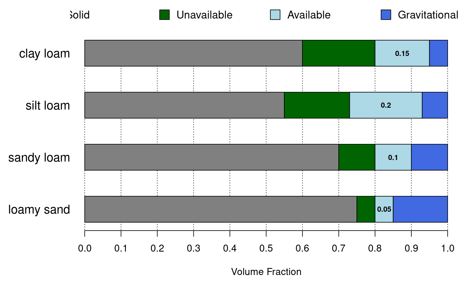
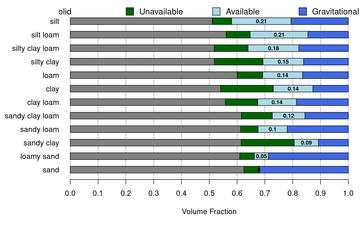
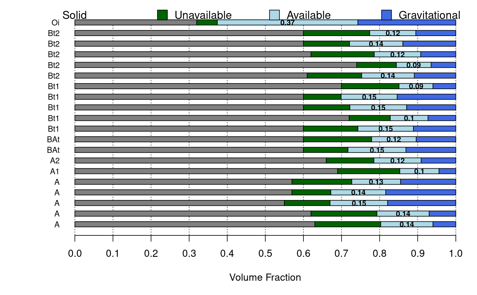
Generate a simplistic diagram of the various fractions of water held within soil pore-space. Largely inspired by Figure 2 from O'Geen (2013).

plotAvailWater(
  x,
  width = 0.25,
  cols = c(grey(0.5), "DarkGreen", "LightBlue", "RoyalBlue"),
  name.cex = 0.8,
  annotate = TRUE
)

Arguments

x

a data.frame containing sample names and water retention data, see examples below

width

vertical width of each bar graph

cols

a vector of colors used to symbolize 'solid phase', 'unavailable water', 'available water', and 'gravitational water'

name.cex

character scaling of horizon names, printed on left-hand side of figure

annotate

logical, annotate AWC

Value

nothing, function is called to generate graphical output

References

O'Geen, A. T. (2013) Soil Water Dynamics. Nature Education Knowledge 4(5):9.

Author

D.E. Beaudette

Examples

# demonstration
s <- data.frame(
  name = c('loamy sand', 'sandy loam', 'silt loam', 'clay loam'), 
  pwp = c(0.05, 0.1, 0.18, 0.2), 
  fc = c(0.1, 0.2, 0.38, 0.35), 
  sat = c(0.25, 0.3, 0.45, 0.4))
s$solid <- with(s, 1-sat)

par(mar=c(5, 6, 0.5, 0.5))
plotAvailWater(s, name.cex=1.25)



# \donttest{
  
  if(requireNamespace("aqp")) {
    
    # demonstration using idealized AWC by soil texture
    data("ROSETTA.centroids", package = "aqp")
    
    # subset columns
    x <- ROSETTA.centroids[, c('texture', 'pwp', 'fc', 'sat', 'awc')]
    
    # adjust to expected names / additional data required by plotAvailWater
    names(x)[1] <- 'name'
    x$solid <- with(x, 1 - sat)
    
    # re-order based on approximate AWC
    x <- x[order(x$awc), ]
    
    op <- par(no.readonly = TRUE)
    
    par(mar=c(5, 6.5, 0.5, 0.5))
    plotAvailWater(x, name.cex = 1)
    
    par(op)
    
  }

  
  
  # use some real data from SSURGO
  if(requireNamespace("curl") &
     curl::has_internet() &
     require(soilDB)) {
    
    q <- "SELECT hzdept_r as hztop, hzdepb_r as hzbottom, 
hzname as name, wsatiated_r/100.0 as sat, 
wthirdbar_r/100.0 as fc, wfifteenbar_r/100.0 as pwp, awc_r as awc
FROM chorizon 
WHERE cokey IN (SELECT cokey from component where compname = 'dunstone') 
AND wsatiated_r IS NOT NULL 
ORDER BY cokey, hzdept_r ASC;"
    
    x <- SDA_query(q)
    x <- unique(x)
    x <- x[order(x$name), ]
    x$solid <- with(x, 1-sat)
    
    op <- par(no.readonly = TRUE)
    
    par(mar=c(5, 5, 0.5, 0.5))
    plotAvailWater(x)
    
    par(op)
  }
#> single result set, returning a data.frame

  
# }