Hue Position Chart

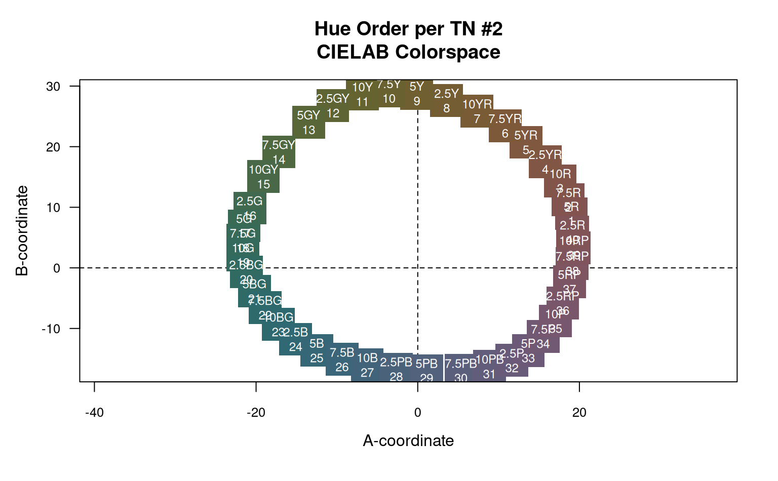
A simple visualization of the hue positions for a given Munsell value/chroma according to Soil Survey Technical Note 2.

huePositionPlot(
  value = 6,
  chroma = 6,
  chip.cex = 4.5,
  label.cex = 0.75,
  contour.dE00 = FALSE,
  origin = NULL,
  origin.cex = 0.75,
  grid.res = 2,
  ...
)

Arguments

value

a single Munsell value

chroma

a single Munsell chroma

chip.cex

scaling for color chip rectangle

label.cex

scaling for color chip

contour.dE00

logical, add dE00 contours from origin, imlpicitly TRUE when origin is not NULL

origin

point used for distance comparisons can be either single row matrix of CIELAB coordinates, a character vector specifying a Munsell color. By default (NULL) represents CIELAB coordinates (L,0,0), where L is a constant value determined by value and chroma. See examples.

origin.cex

scaling for origin point

grid.res

grid resolution for contours, units are CIELAB A/B coordinates. Caution, small values result in many pair-wise distances which could take a very long time.

...

additional arguments to contour()

Value

nothing, function is called to generate graphical output

Examples

# \donttest{
# adjust Munsell value and chroma for all hues
huePositionPlot(value = 4, chroma = 4)

# huePositionPlot(value = 6, chroma = 6)
# huePositionPlot(value = 8, chroma = 8)

## contour dE00 values from CIELBA (A,B) origin
# huePositionPlot(value = 6, chroma = 6, contour.dE00 = TRUE, grid.res = 2)

## shift origin to arbitrary CIELAB coordinates or Munsell color
# huePositionPlot(origin = cbind(40, 5, 15), origin.cex = 0.5)

# huePositionPlot(origin = '5G 6/4', origin.cex = 0.5)

# huePositionPlot(origin = '10YR 3/4', origin.cex = 0.5)

# huePositionPlot(value = 3, chroma = 4, origin = '10YR 3/4', origin.cex = 0.5)

# }