Plot Aspect Data

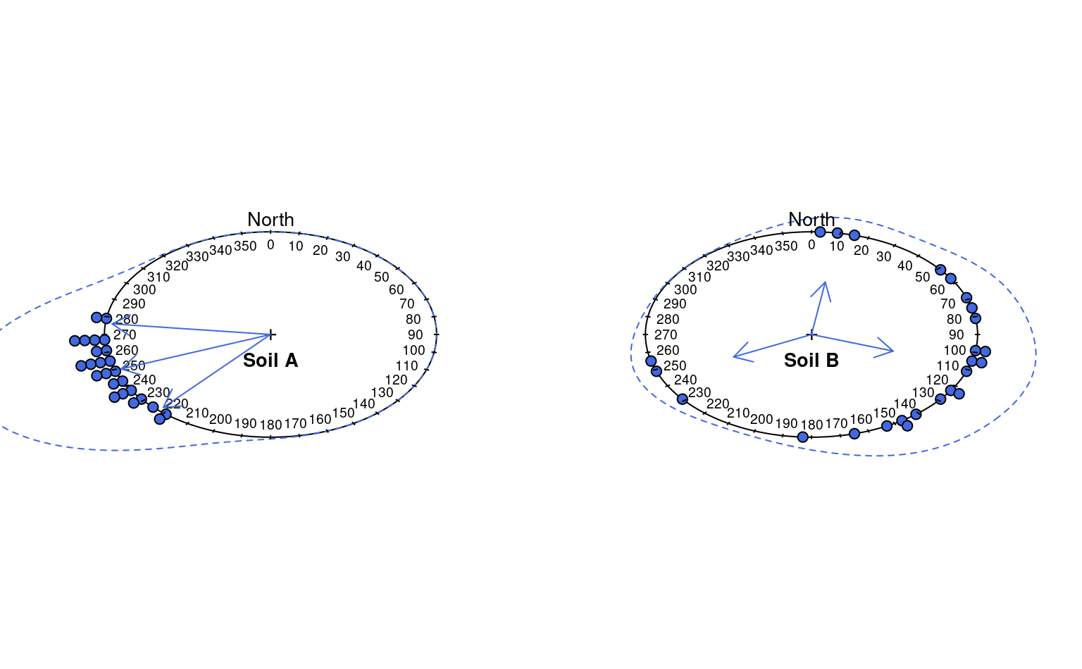
Plot a graphical summary of multiple aspect measurements on a circular diagram.

aspect.plot(
  p,
  q = c(0.05, 0.5, 0.95),
  p.bins = 60,
  p.bw = 30,
  stack = TRUE,
  p.axis = seq(0, 350, by = 10),
  plot.title = NULL,
  line.col = "RoyalBlue",
  line.lwd = 1,
  line.lty = 2,
  arrow.col = line.col,
  arrow.lwd = 1,
  arrow.lty = 1,
  arrow.length = 0.15,
  ...
)

Arguments

p

a vector of aspect angles in degrees, measured clock-wise from North

q

a vector of desired quantiles

p.bins

number of bins to use for circular histogram

p.bw

bandwidth used for circular density estimation

stack

logical, should the individual points be stacked into p.bins number of bins and plotted

p.axis

a sequence of integers (degrees) describing the circular axis

plot.title

an informative title

line.col

density line color

line.lwd

density line width

line.lty

density line line style

arrow.col

arrow color

arrow.lwd

arrow line width

arrow.lty

arrow line style

arrow.length

arrow head length

...

further arguments passed to circular::plot.circular

Value

invisibly returns circular stats

Details

Spread and central tendency are depicted with a combination of circular histogram and kernel density estimate. The circular mean, and relative confidence in that mean are depicted with an arrow: longer arrow lengths correspond to greater confidence in the mean.

Note

Manual adjustment of p.bw may be required in order to get an optimal circular density plot. This function requires the package circular, version 0.4-7 or later.

Author

D.E. Beaudette

Examples

# simulate some data
p.narrow <- runif(n=25, min=215, max=280)
p.wide <- runif(n=25, min=0, max=270)

# set figure margins to 0, 2-column plot
op <- par(no.readonly = TRUE)
par(mar = c(0,0,0,0), mfcol = c(1,2))

# plot, save circular stats 
x <- aspect.plot(p.narrow, p.bw=10, plot.title='Soil A', pch=21, col='black', bg='RoyalBlue')
y <- aspect.plot(p.wide, p.bw=10, plot.title='Soil B', pch=21, col='black', bg='RoyalBlue')


# reset output device options
par(op) 

x
#> Circular Data: 
#> Type = angles 
#> Units = degrees 
#> Template = geographics 
#> Modulo = 2pi 
#> Zero = 1.570796 
#> Rotation = clock 
#>       5%      50%      95% 
#> 276.1947 249.5523 222.2640 
#> attr(,"uniformity")
#> Rayleigh Uniformity             p Value 
#>        9.593211e-01        5.520616e-10