Soil Morphologic, Geochemical, and Mineralogy Data from Rowley et al. 2019.

Data from Table 1 and Supplementary Tables 1 and 2 from "A cascading influence of calcium carbonate on the biogeochemistry and pedogenic trajectories of subalpine soils, Switzerland".

data(rowley2019)

Format

A SoilProfileCollection object:

site-level attributes

id: profile ID
group: profile group

horizon-level attributes

sample_id: sample ID
name: horizon name
pH: pH
Al_exch: cmol(+) / kg, exchangeable Al
Ca_exch: cmol(+) / kg, exchangeable Ca
CEC_sum: cmol(+) / kg, cation exchange capacity calculated as the sum of exchangeable cations, not including H+
Ca_exch_saturation: percent
Al_exch_saturation: percent
TON: percent, total nitrogen
SOC: percent, soil organic carbon
C_to_N: carbon to nitrogen ratio
Alo: g/kg, oxalate-extractable Al
Feo: g/kg, oxalate-extractable Fe
Ald: g/kg, dithionite-extractable Al
Fed: g/kg, dithionite-extractable Fe
Feo_Fed: Fe_o to Fe_d ratio
id: profile ID
top: horizon top (cm)
bottom: horizon bottom (cm)
Al: g/kg by x-ray fluorescence
Ca: g/kg by x-ray fluorescence
Cr: g/kg by x-ray fluorescence
Fe: g/kg by x-ray fluorescence
K: g/kg by x-ray fluorescence
Mg: g/kg by x-ray fluorescence
Mn: g/kg by x-ray fluorescence
Na: g/kg by x-ray fluorescence
Ni: g/kg by x-ray fluorescence
P: g/kg by x-ray fluorescence
Si: g/kg by x-ray fluorescence
Ti: g/kg by x-ray fluorescence
Phyllosilicates: percent by x-ray diffraction spectra
Quartz: percent by x-ray diffraction spectra
K_Feldspar: percent by x-ray diffraction spectra
Na_Plagioclase: percent by x-ray diffraction spectra
Goethite: percent by x-ray diffraction spectra
Unidentified: percent by x-ray diffraction spectra
CCE_Total: percent
CCE_Reactive: percent
Reactive_carbonate: percent
Sand: percent <2um
Silt: percent 2-50um
Clay: percent 50-2000um
CaH2O: Milliq ex: grams of Ca per kilogram of dry soil (g kg-1)
Ca2MKCl: 2M KCl: grams of Ca per kilogram of dry soil (g kg-1)
CaNa2EDTA: 0.05 M Na2EDTA: grams of Ca per kilogram of dry soil (g kg-1)
CaCuCl2: 0.5 M CuCl2: grams of Ca per kilogram of dry soil (g kg-1)
hzID: horizon ID

References

Mike C. Rowley, Stephanie Grand, Thierry Adatte, Eric P. Verrecchia, Cascading influence of calcium carbonate on the biogeochemistry and pedogenic trajectories of subalpine soils), Switzerland, Geoderma, 2019, 114065, ISSN 0016-7061, doi:10.1016/j.geoderma.2019.114065 .

Examples


library(lattice)

# load data
data('rowley2019')

# check first 5 rows and 10 columns of horizon data
horizons(rowley2019)[1:5, 1:10]
#>   sample_id name  pH Al_exch Ca_exch CEC_sum Ca_exch_saturation
#> 1      B1.1  Ah1 6.3       0    23.2    23.7               97.6
#> 2      B1.2  Ah2 6.4       0    23.0    23.4               98.4
#> 3      B1.3  ABh 6.3       0    20.3    20.6               98.5
#> 4      B1.4   Bh 6.4       0    16.9    17.2               98.4
#> 5      B1.5   B1 6.4       0    15.2    15.5               98.3
#>   Al_exch_saturation TON SOC
#> 1                  0 0.8 7.7
#> 2                  0 0.8 6.8
#> 3                  0 0.6 5.3
#> 4                  0 0.5 4.3
#> 5                  0 0.4 3.4

# check site data
site(rowley2019)
#>   id          group
#> 1 B1 CaCO3-bearing 
#> 2 B2 CaCO3-bearing 
#> 3 B3 CaCO3-bearing 
#> 4 F1     CaCO3-free
#> 5 F2     CaCO3-free
#> 6 F3     CaCO3-free

# graphical summary
par(mar=c(1,1,3,1))
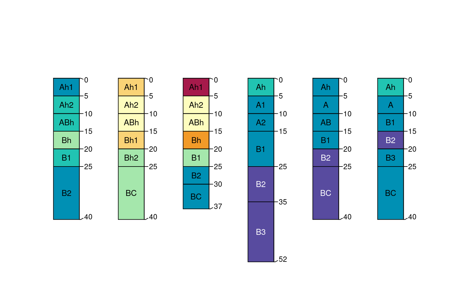
plotSPC(rowley2019, color='Feo_Fed', name='name', cex.names=0.85)


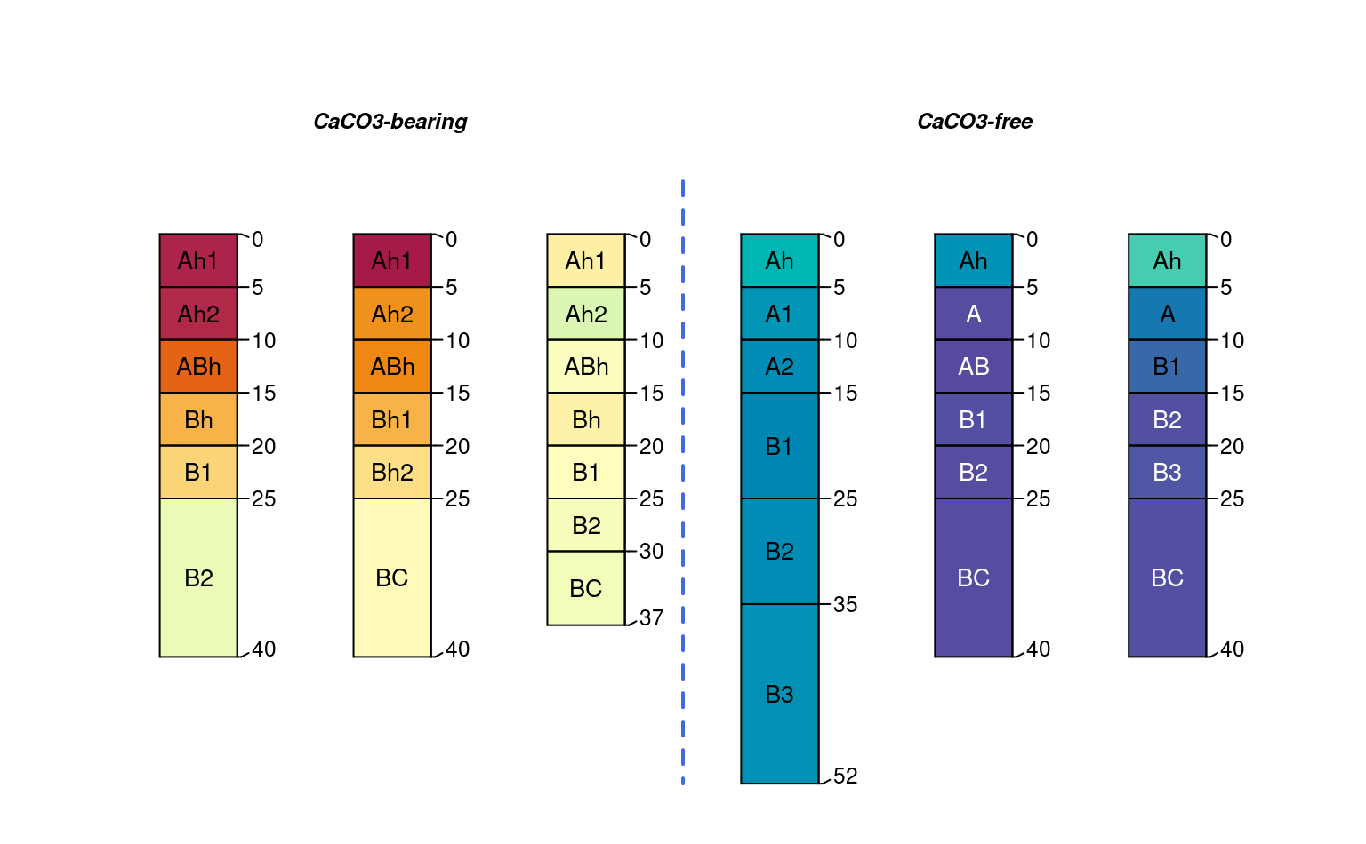
plotSPC(rowley2019, color='Ca_exch', name='name', cex.names=0.85)

# grouped plot
groupedProfilePlot(rowley2019, groups = 'group', color='Ca_exch',
name='name', cex.names=0.85, group.name.offset = -10)


# aggregate over 1cm slices, for select properties
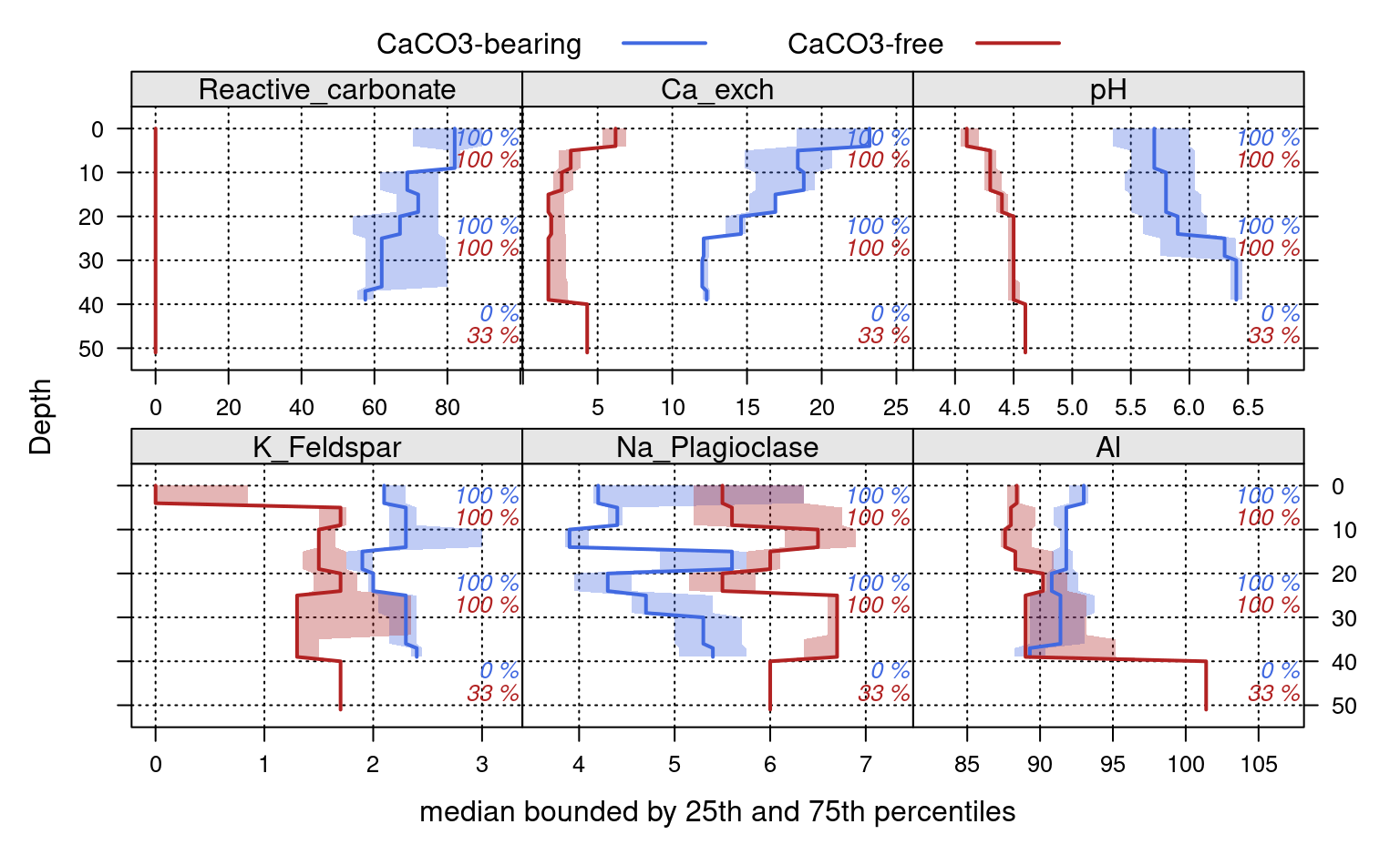
a <- slab(rowley2019, group ~ Reactive_carbonate + Ca_exch + pH + K_Feldspar + Na_Plagioclase + Al)

# plot styling
tps <- list(superpose.line=list(lwd=2, col=c('royalblue', 'firebrick')))

# make the figure
xyplot(top ~ p.q50 | variable, data=a, ylab='Depth', groups=group,
       main='', as.table=TRUE,
       xlab='median bounded by 25th and 75th percentiles',
       lower=a$p.q25, upper=a$p.q75, ylim=c(55,-5),
       panel=panel.depth_function,
       prepanel=prepanel.depth_function,
       cf=a$contributing_fraction,
       alpha=0.33, sync.colors=TRUE,
       scales=list(x=list(relation='free', alternating=1)),
       par.settings=tps,
       auto.key=list(columns=2, lines=TRUE, points=FALSE),
       strip=strip.custom(bg=grey(0.9))
)