Example SoilProfilecollection Objects Returned by fetchNASIS.

Several examples of soil profile collections returned by fetchNASIS(from='pedons') as SoilProfileCollection objects.

Examples

# \donttest{
# load example dataset
  data("gopheridge")

  # what kind of object is this?
  class(gopheridge)
#> [1] "SoilProfileCollection"
#> attr(,"package")
#> [1] "aqp"

  # how many profiles?
  length(gopheridge)
#> [1] 52

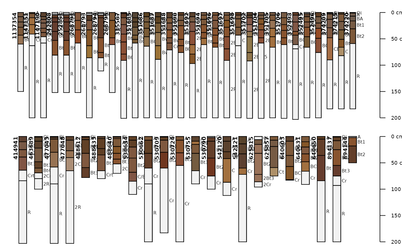
  # there are 60 profiles, this calls for a split plot
  par(mar=c(0,0,0,0), mfrow=c(2,1))

  # plot soil colors
  plot(gopheridge[1:30, ], name='hzname', color='soil_color')
  plot(gopheridge[31:60, ], name='hzname', color='soil_color')


  # need a larger top margin for legend
  par(mar=c(0,0,4,0), mfrow=c(2,1))
  # generate colors based on clay content
  plot(gopheridge[1:30, ], name='hzname', color='clay')
  plot(gopheridge[31:60, ], name='hzname', color='clay')


  # single row and no labels
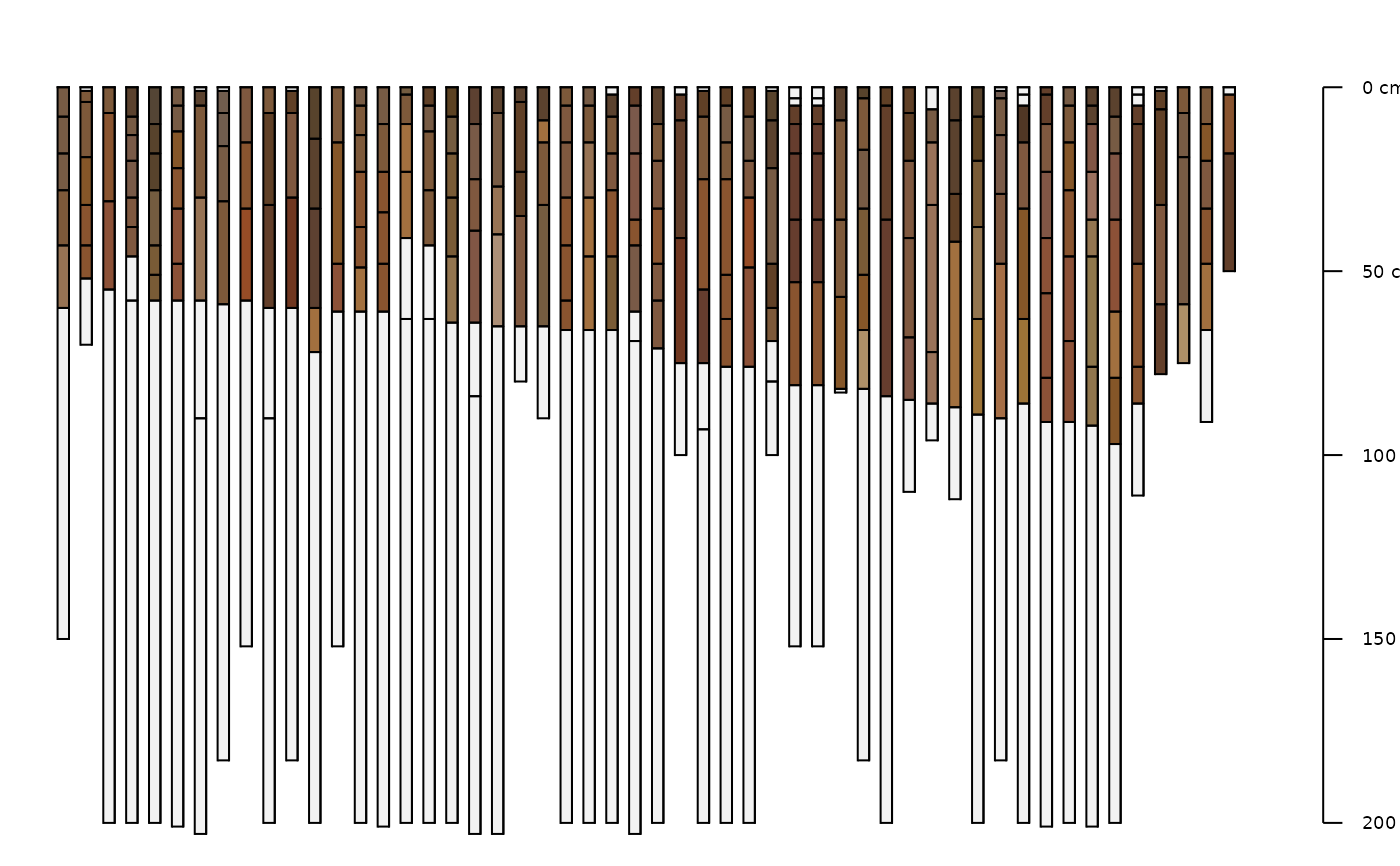
  par(mar=c(0,0,0,0), mfrow=c(1,1))
  # plot soils sorted by depth to contact
  plot(gopheridge, name='', print.id=FALSE, plot.order=order(gopheridge$bedrckdepth))


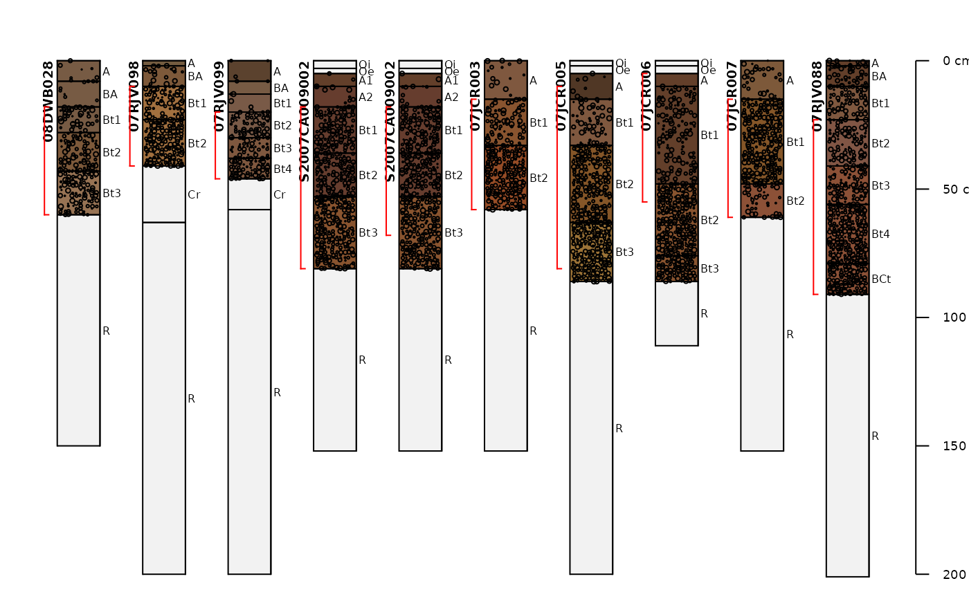
  # plot first 10 profiles
  plot(gopheridge[1:10, ], name='hzname', color='soil_color', label='pedon_id', id.style='side')

  # add rock fragment data to plot:
  addVolumeFraction(gopheridge[1:10, ], colname='total_frags_pct')

  # add diagnostic horizons
  addDiagnosticBracket(gopheridge[1:10, ], kind='argillic horizon', col='red', offset=-0.4)


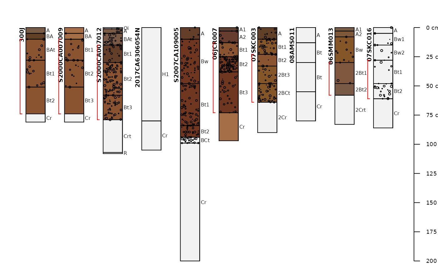
  ## loafercreek
  data("loafercreek")
  # plot first 10 profiles
  plot(loafercreek[1:10, ], name='hzname', color='soil_color', label='pedon_id', id.style='side')

  # add rock fragment data to plot:
  addVolumeFraction(loafercreek[1:10, ], colname='total_frags_pct')

  # add diagnostic horizons
  addDiagnosticBracket(loafercreek[1:10, ], kind='argillic horizon', col='red', offset=-0.4)

# }