Bootstrap Soil Texture Data

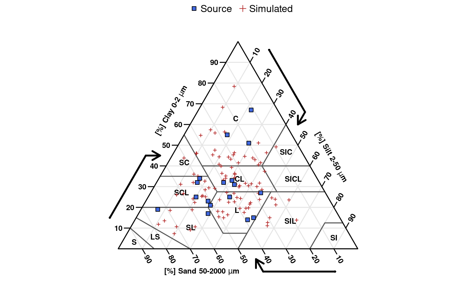
Simulate realistic sand/silt/clay values (a composition) using multivariate Normal distribution or Dirichlet distribution. Simulations from the multivariate Normal distribution are based on the compositional mean and variance-covariance matrix. Simulations from the Dirichlet distribution are based on maximum likelihood estimation of alpha parameters.

bootstrapSoilTexture(ssc, method = c("dirichlet", "normal"), n = 100)

Arguments

ssc

a data.frame object with 3 columns: 'sand', 'silt', 'clay' and at least three rows of data within the range of 0-100 (percent). NA are automatically removed, but care should be taken to ensure that the sand/silt/clay values add to 100 percent. Simulations are based on these examples.

method

type of simulation: 'dirichlet' or 'normal'. See details.

n

number of simulated compositions. See details.

Value

a list containing:

• samples - data.frame of simulated sand, silt, clay values

• mean - compositional mean

• var - compositional variance-covariance matrix

• D.alpha - (fitted) alpha parameters of the Dirichlet distribution, NULL when method = 'normal'

Details

Simulations from the multivariate normal distribution will more closely track the marginal distributions of sand, silt, and clay–possibly a better fit for "squished" compositions (TODO elaborate). However, these simulations can result in extreme (unlikely) estimates.

Simulations from the Dirichlet distribution will usually be a better fit (fewer extreme estimates) but require a fairly large number of records in ssc (n >= 30?) for a reliable fit.

Additional examples will be added to this tutorial.

References

Aitchison, J. (1986) The Statistical Analysis of Compositional Data Monographs on Statistics and Applied Probability. Chapman & Hall Ltd., London (UK). 416p.

Aitchison, J, C. Barcel'o-Vidal, J.J. Egozcue, V. Pawlowsky-Glahn (2002) A concise guide to the algebraic geometric structure of the simplex, the sample space for compositional data analysis, Terra Nostra, Schriften der Alfred Wegener-Stiftung, 03/2003

Malone Brendan, Searle Ross (2021) Updating the Australian digital soil texture mapping (Part 1*): re-calibration of field soil texture class centroids and description of a field soil texture conversion algorithm. Soil Research. https://www.publish.csiro.au/SR/SR20283

Malone Brendan, Searle Ross (2021) Updating the Australian digital soil texture mapping (Part 2*): spatial modelling of merged field and lab measurements. Soil Research. https://doi.org/10.1071/SR20284

Author

D.E. Beaudette

Examples

# \donttest{
if(
requireNamespace("compositions") &
  requireNamespace("soiltexture")
) {
  
  # sample data, data.frame
  data('sp4')
  
  # filter just Bt horizon data
  ssc <- sp4[grep('^Bt', sp4$name), c('sand', 'silt', 'clay')]
  names(ssc) <- toupper(names(ssc))
  
  # simulate 100 samples
  s <- bootstrapSoilTexture(ssc, n = 100)
  s <- s$samples
  
  # empty soil texture triangle
  TT <- soiltexture::TT.plot(
    class.sys= "USDA-NCSS.TT",
    main= "",
    tri.sum.tst=FALSE,
    cex.lab=0.75,
    cex.axis=0.75,
    frame.bg.col='white',
    class.lab.col='black',
    lwd.axis=1.5,
    arrows.show=TRUE,
    new.mar = c(3, 0, 0, 0)
  )
  
  # add original data points
  soiltexture::TT.points(
    tri.data = s, geo = TT, col='firebrick', 
    pch = 3, cex = 0.5, lwd = 1, 
    tri.sum.tst = FALSE
  )
  
  # add simulated points
  soiltexture::TT.points(
    tri.data = ssc, geo = TT, bg='royalblue', 
    pch = 22, cex = 1, lwd = 1, 
    tri.sum.tst = FALSE
  )
  
  # simple legend
  legend('top', 
         legend = c('Source', 'Simulated'), 
         pch = c(22, 3), 
         col = c('black', 'firebrick'), 
         pt.bg = c('royalblue', NA), 
         horiz = TRUE, bty = 'n'
  )
  
  
}
#> Loading required namespace: compositions
#> Loading required namespace: soiltexture
#> Warning: no DISPLAY variable so Tk is not available


# }